kd tree construction using the surface area heuristic, stack-based traversal, and the hyperplane separation theorem

In this post we will employ the hyperplane separation theorem and the surface area heuristic for kd tree construction to improve the performance of our path tracer. Previous posts have relied simply on detecting intersections between an axis aligned bounding box and the minimum bounding box of a triangle primitive. By utilizing the hyperplane separation theorem, we can cull additional triangles from a list of potential intersection candidates. From here, we will set out to construct a kd tree using the surface area heuristic. The construction method we will implement has complexity, \(O(n \cdot \log^2n)\). Finally, we will implement a stack-based kd tree traversal algorithm.

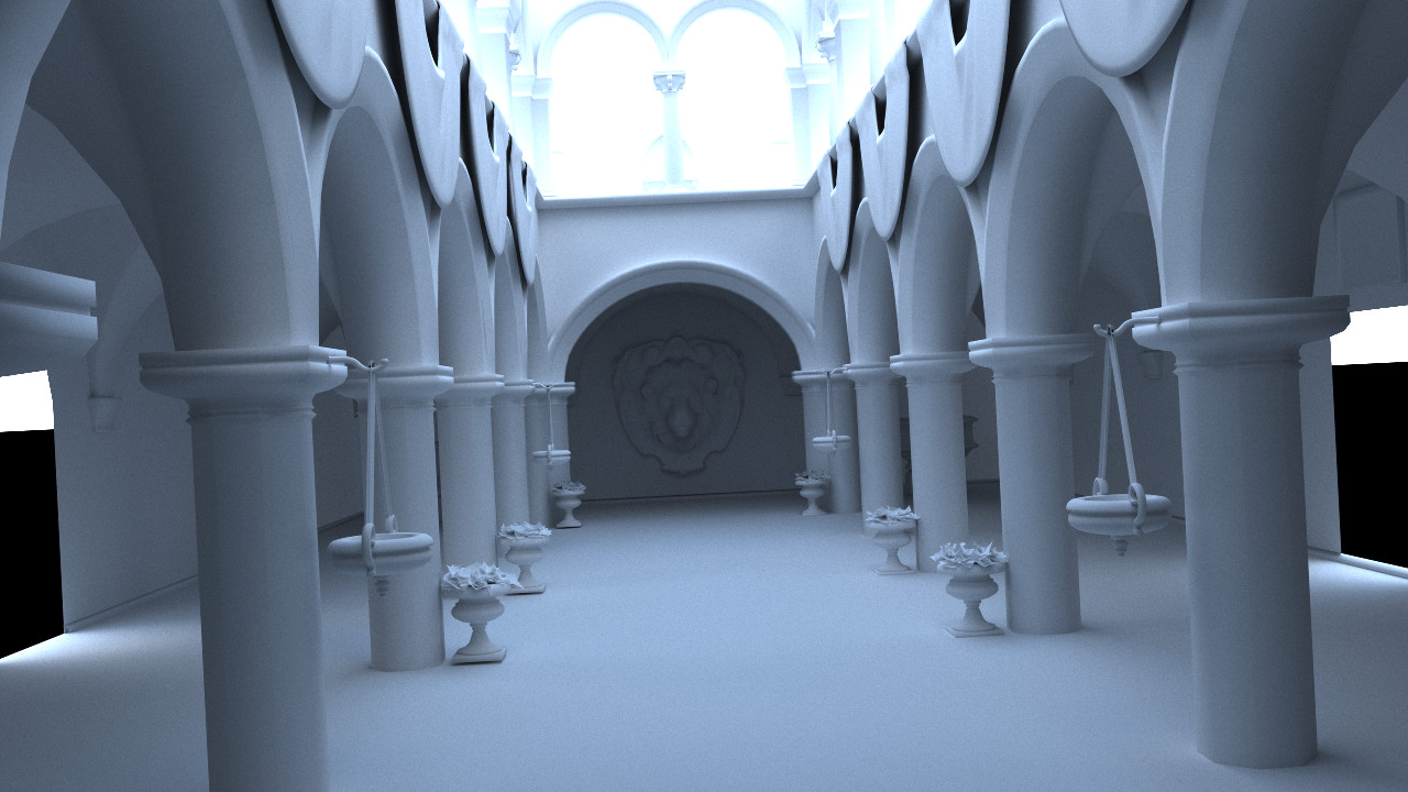
Below is a test render of the Sponza model. Some of the features of the original model have been stripped for this render, leaving approximately 150,000 triangles.

Below is a render of the Dragon model available from the Stanford 3D Scanning Repository. The rendered model contained 100,000 triangles.

Hyperplane Separation Theorem
The hyperplane separation theorem is a theorem about disjoint, convex sets. For our purposes we will be applying the theorem to a combination of an axis-aligned bounding box and a triangle in three dimensions. Since we will consider both the triangle and the axis-aligned bounding box to be compact (and convex), then, provided these two sets are disjoint, we can locate two parallel hyperplanes between them separated by a gap. We need only one separating hyperplane to conclude that the triangle and axis-aligned bounding box do not intersect. Below is an image depicting this theorem in two dimensions. The green line is a separating axis and the black line is a separating line.

In three dimensions, we will have a separating axis and a separating plane. We have a few different contact situations between objects to concern ourselves with: face to face contact, face to edge contact, and edge to edge contact. Thus, we have a list of potential separating axes including the normals to the faces and the cross products of the combinations of an edge from one object with an edge from the other. The face to edge contacts are handled by the face normals. The axis-aligned bounding box has six faces, but three sets of two parallel faces, so we have three potential separating axes. The triangle normal is a fourth. The axis-aligned bounding box has 12 edges, but three sets of four parallel edges, and the triangle has three edges, yielding nine cross products for a total of 13 potential separating axes. We need only complete all thirteen tests to conclude that the axis-aligned bounding box and the triangle are not disjoint. However, if any particular tests yields a separating plane, we need not complete the remaining tests to conclude that the objects are disjoint.

We will first translate the triangle and the axis-aligned bounding box such that the center of the box is located at the origin. Below is some code to detect a separation. We need not be concerned with the direction of the projections, but only their magnitudes. Because the box is located at the origin, we define a radius, r, based on the half dimensions of the box.

bool hyperplaneSeparation(__vector n,
		          __vector p0, __vector p1, __vector p2,
		          double halfWidth, double halfHeight, double halfDepth) {
	double _p0 = n * p0,
	       _p1 = n * p1,
	       _p2 = n * p2;
	double min = MIN(_p0, MIN(_p1, _p2)),
	       max = MAX(_p0, MAX(_p1, _p2));
	double r = halfWidth  * fabs(n.x) +
	           halfHeight * fabs(n.y) +
	           halfDepth  * fabs(n.z);
	return -r > max || r < min;
}

The buildTree() function in the project download uses this method.

kd tree construction using the surface area heuristic
kd tree construction using the surface area heuristic is a greedy algorithm. During the build process, we will attempt to compare the cost of splitting a node with the cost of not splitting. If the local cost of splitting is less than not splitting, we split the node. Otherwise, we convert the current node to a leaf. The function we will use to estimate the cost is given below [2],
\begin{align}
C_V(p) &= K_T + K_I\left( \frac{SA(V_L)}{SA(V)} T_L + \frac{SA(V_R)}{SA(V)} T_R \right) \\
C_{NS} &= K_IT \\
\end{align}
where \(K_T\) is the cost of a traversal, \(K_I\) is the triangle intersection cost, \(SA(V_L), SA(V_R), SA(V)\) are the surface areas of the left node, right node, and current node, respectively, \(T_L, T_R, T\) are the number of triangles in the left node, right node, and current node, respectively, \(C_V(p)\) is the cost of splitting the current node, and \(C_{NS}\) is the cost of not splitting the current node.

We have \(6T\) potential split positions comprising each of the three axes with the minimum and maximum value for each axis from each triangle. The algorithm presented here is similar to the \(O(n \cdot \log^2n)\) algorithm described in [2]. For each axis we push the minimum triangle coordinate to a list with an event, PRIMITIVE_START, and the maximum coordinate with an event, PRIMITIVE_END. The lists are then sorted based on the coordinate value, \(O(n \cdot \log n)\). For each split position, we will consider the triangle to reside in both nodes, so for the first split position we have \(T_L=1\) and \(T_R=T\). As we progress to the next split position, if that event is a PRIMITIVE_START, we increment \(T_L\). If the event is a PRIMITIVE_END, we decrement \(T_R\) on the following pass, since that event corresponds to a triangle that we are including in both nodes (a vertex lies on the split plane). We now have \(T_L\) and \(T_R\) for each split position, we can evaluate the surface areas based on the split position, and throw some estimates in for \(K_T\) and \(K_I\). On each pass we evaluate \(C_V(p)\) and retain the best cost and split position, \(p\). Once we have processed all potential split positions, we compare the best cost with \(C_{NS}\) and split the node if \(C_V(p) \lt C_{NS}\).

The project download generates the kd tree recursively host-side, transfers it to a structure of arrays, and passes it to the device. The buildKdTree() function in the download allows you to pass a type parameter. This parameter can be KD_EVEN, splitting each node in the center resulting in a binary space partition, KD_MEDIAN, splitting each node at the object median, or KD_SAH, splitting the node using surface area heuristics. Below are three visualizations of the tree structure for each type.

stack-based traversal
To implement a stack-based traversal of the kd tree, we first created a stack object below. The __stack_element contains an id to reference a node, and the \(t_{min}\) and \(t_{max}\) values for a ray, \(\vec{r} = \vec{o} + \hat{d}t\), passing through the node.

struct __stack_element {
	int id;
	double tmin, tmax;
};

class __stack {
public:
	__stack_element stack[32];
	int count;
	__device__ __stack();
	__device__ void push(int id, double tmin, double tmax);
	__device__ __stack_element pop();
	__device__ bool empty();
};

__device__ __stack::__stack() : count(0) {}

__device__ void __stack::push(int id, double tmin, double tmax) {
	this->stack[count].id = id;
	this->stack[count].tmin = tmin;
	this->stack[count].tmax = tmax;
	count++;
}

__device__ __stack_element __stack::pop() {
	count--;
	__stack_element se;
	se.id = this->stack[count].id;
	se.tmin = this->stack[count].tmin;
	se.tmax = this->stack[count].tmax;
	return se;
}

__device__ bool __stack::empty() {
	return this->count == 0;
}

With the stack object, it was fairly straightforward to implement the algorithm below. See [3] and [4] for details. The algorithm descends through the tree, pushing the further nodes onto the stack. With the nearest nodes evaluated first, we can break early upon finding an intersection within the bounds.

intersection = none;
if (ray intersects root node) {
    stack.push(root node, tmin, tmax);
    while (!stack.empty() && !intersection) {
        (node, tmin, tmax) = stack.pop();
        while (!node.isLeaf()) {
            tsplit = (node.split - ray.origin[node.axis]) / ray.direction[node.axis];
            if (node.split - ray.origin[node.axis] >= 0) {
                first = node.left;
                second = node.right;
            } else {
                first = node.right;
                second = node.left;
            }
            if (tsplit >= tmax || tsplit < 0)
                node = first;
            else if (tsplit <= tmin)
                node = second;
            else {
                stack.push(second, tsplit, tmax);
                node = first;
                tmax = tsplit;
            }
        }
        foreach (triangle in node)
            if (ray intersects triangle)
                intersection = nearest intersection;
        if (nearest intersection > tmax)
                intersection = none;
    }
}

Download the project and have a look at the code. Let me know if you have any thoughts.

Download this project: path_tracer.tar.bz2

References:
1. Akenine-Möller, Tomas. Fast 3D triangle-box overlap testing. In ACM SIGGRAPH 2005 Courses, ACM. Los Angeles, California. 2005.
2. Wald, Ingo, and Havran, Vlastimil. On building fast kd-Trees for Ray Tracing, and on doing that in O(N log N). IN PROCEEDINGS OF THE 2006 IEEE SYMPOSIUM ON INTERACTIVE RAY TRACING. 2006.
3. Wald, Ingo. 2004. Realtime Ray Tracing and Interactive Global Illumination. PhD thesis, Saarland University.
4. Horn, Daniel Reiter, Sugerman, Jeremy, Houston, Mike, and Hanrahan, Pat. 2007. Interactive k-d tree GPU raytracing. In Proceedings of the 2007 symposium on Interactive 3D graphics and games, ACM. Seattle, Washington.
5. Havran, Vlastimil. 2000. Heuristic Ray Shooting Algorithms. Ph.D. Thesis, Czech Technical University in Prague.