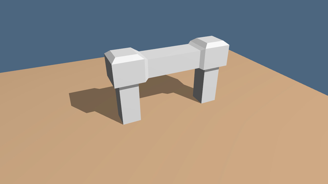
The purpose of this project was to provide a straightforward implementation of shadow volumes using the depth fail approach. The project is divided into the following sections: After loading an object, detect duplicate vertices. Build the object's edge list while identifying each face associated with an edge. Identify the profile edges from the perspective of …
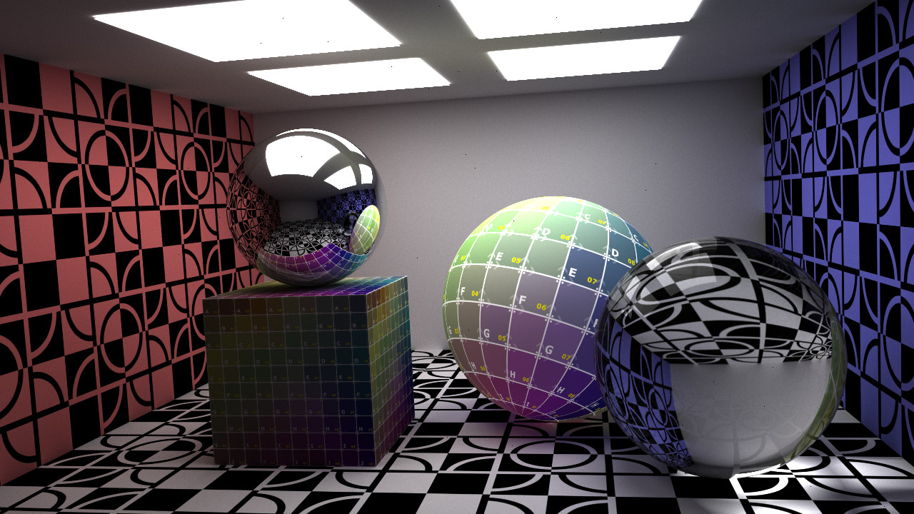
I had been planning to refine this project and offer a more detailed writeup on adding sphere and triangle texture mapping to the path tracer project, but for the time being I thought I would offer the code for download. Below are a couple of screen captures from the most recent version of the project. …
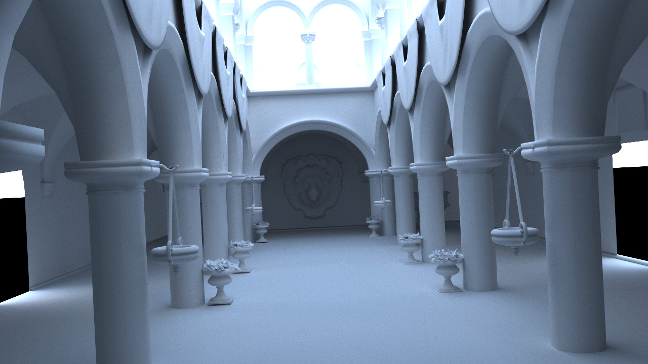
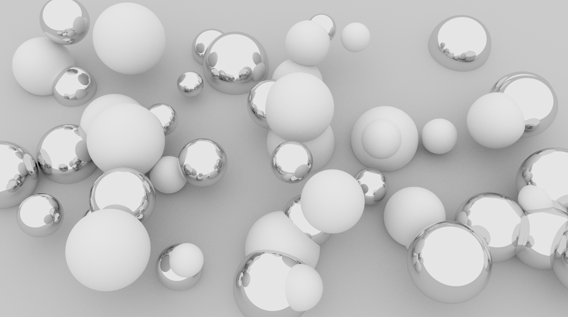
In this post we will employ the hyperplane separation theorem and the surface area heuristic for kd tree construction to improve the performance of our path tracer. Previous posts have relied simply on detecting intersections between an axis aligned bounding box and the minimum bounding box of a triangle primitive. By utilizing the hyperplane separation …
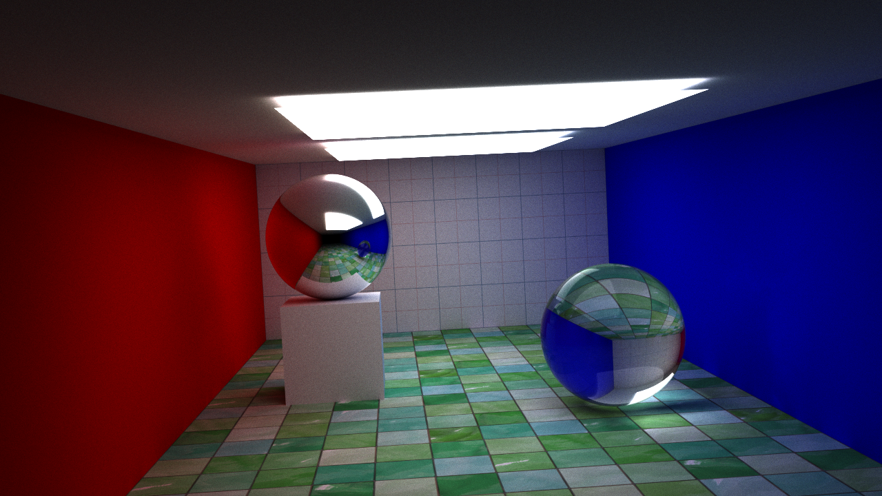
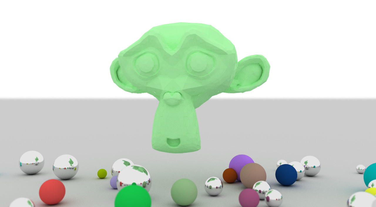
A few new features have been added to our path tracer. The depth of field extension has been reworked slightly using the thin lens equation allowing us to specify a focal length and aperture. Fresnel equations have been added to more accurately model the behavior of light at the interface between media of different refractive …
UPDATE: The post below was a purely naive attempt at implementing a rudimentary bounding volume hierarchy. A much more efficient implementation using a kd tree is available in this post. We will continue with the project we left off with in this post. We will attempt to add triangles to our list of primitives. Once …
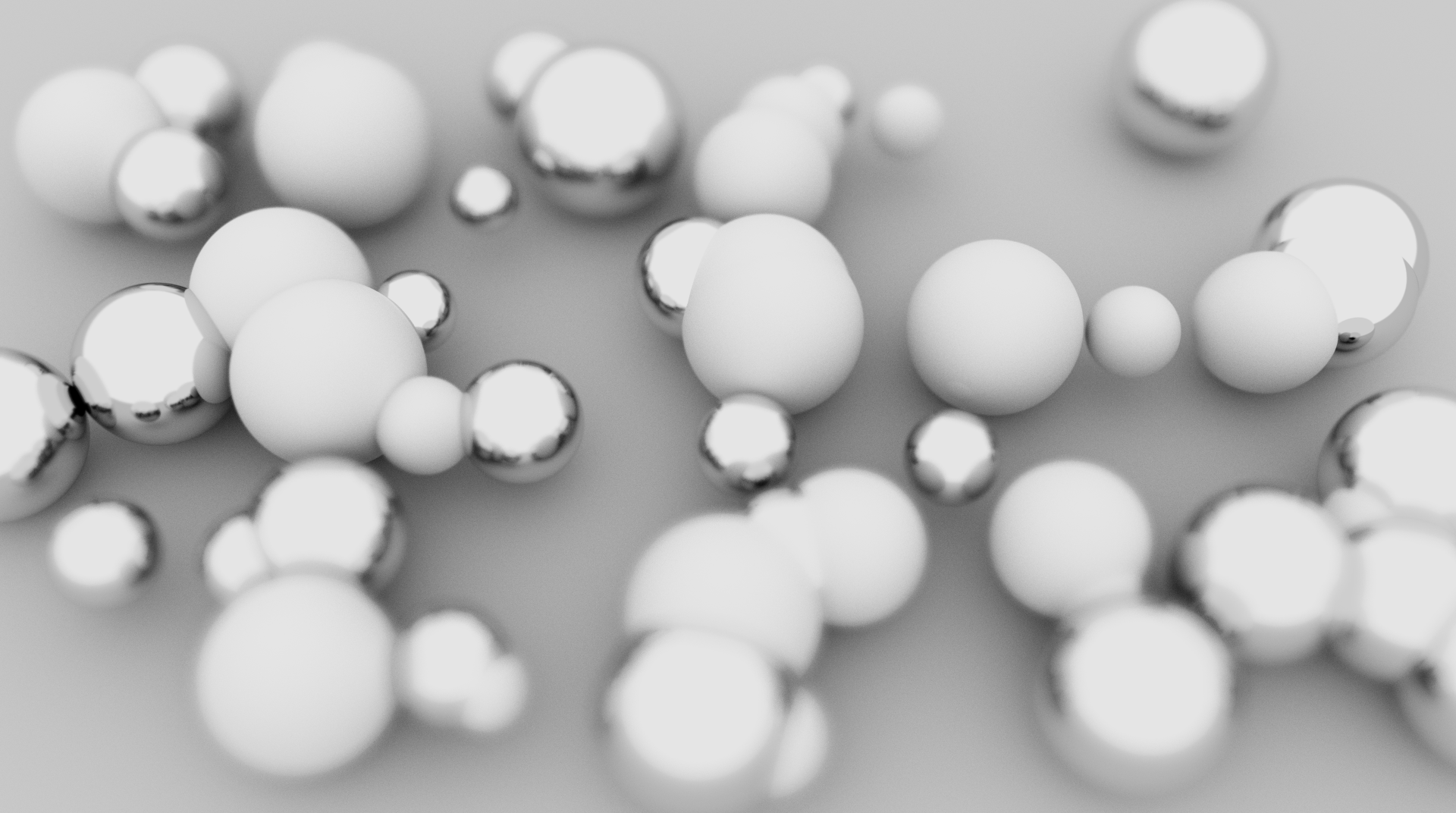
This is a small extension to the previous post. We will add a depth of field simulation to our path tracer project. I ran across this algorithm at this site. Below is a render of our path tracer with the depth of field extension. Essentially, we will define the distance to the focal plane and …
The path tracer we will create in this project will run on CUDA-enabled GPUs. You will need to install the CUDA Toolkit available from NVIDIA. The device code for this project uses classes and must be compiled with compute capability 2.0. If you are unsure what compute capability your card has, check out this list. …
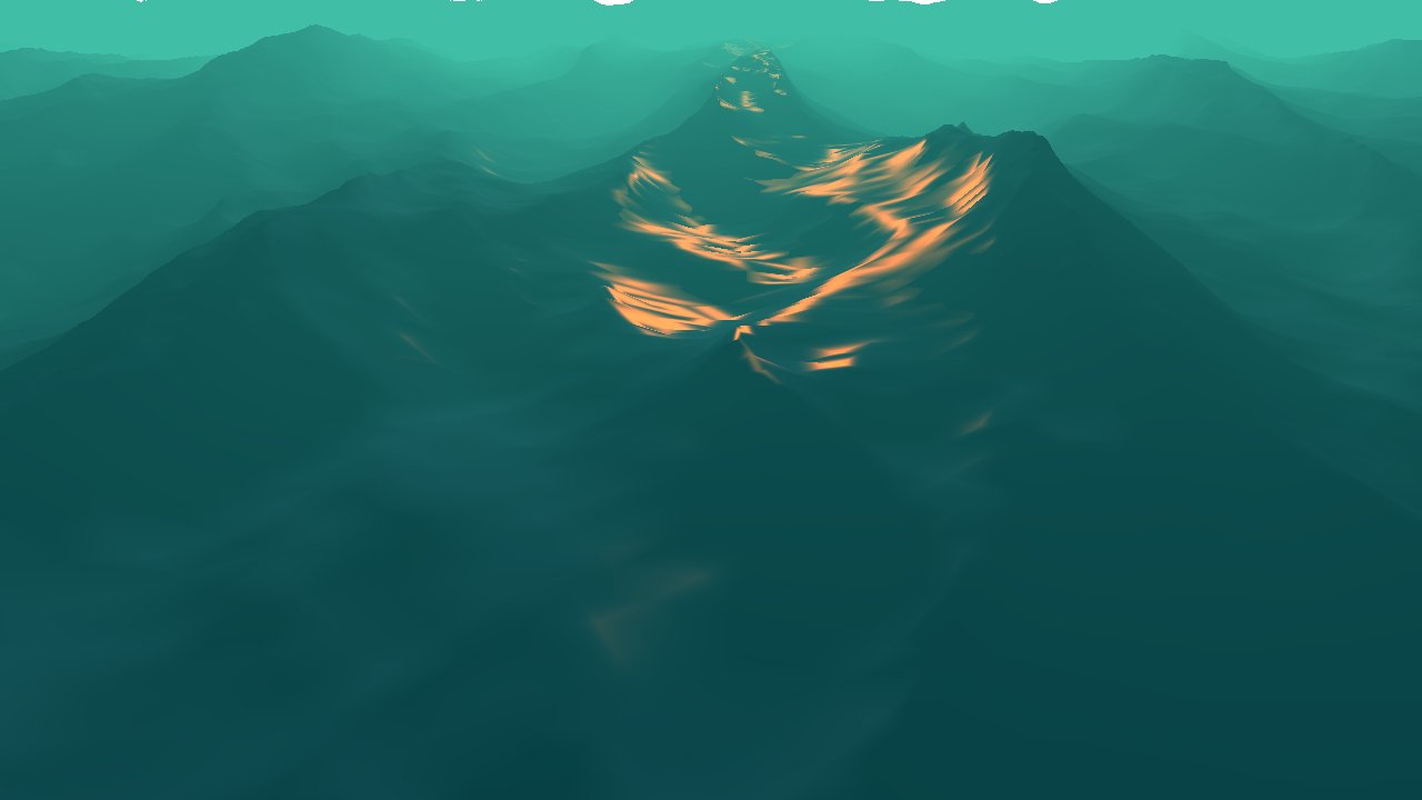
In this post we will analyze the equations for the statistical wave model presented in Tessendorf's paper[1] on simulating ocean water. In the previous post we used the discrete Fourier transform to generate our wave height field. We will proceed with the analysis in order to implement our own fast Fourier transform. With this implementation …
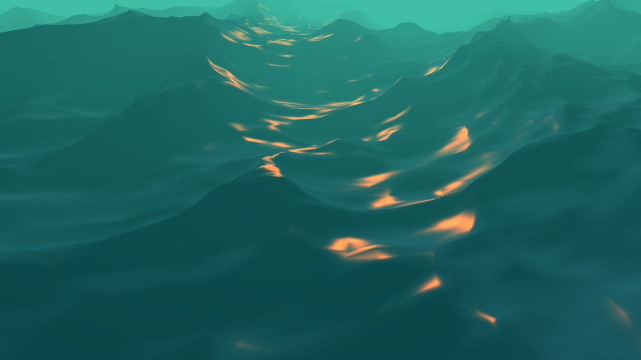
In this post we will implement the statistical wave model from the equations in Tessendorf's paper[1] on simulating ocean water. We will implement this model using a discrete Fourier transform. In part two we will begin with the same equations but provide a deeper analysis in order to implement our own fast Fourier transform. Using …
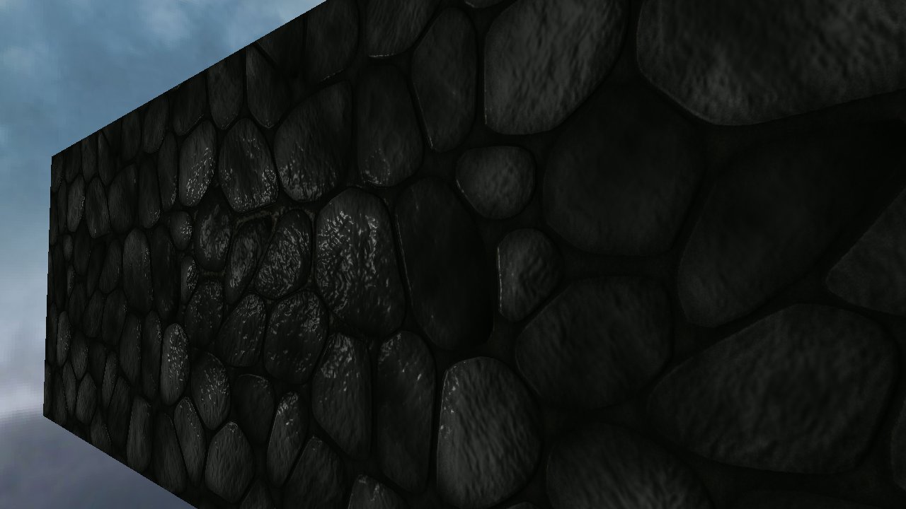
In the previous post we discussed lighting and environment mapping, and our evaluation of the lighting contribution was performed in view space. Here we will discuss lighting in tangent space and extend our lighting model to include a normal map. If we apply a texture to a surface, then for every point in the texture …

In this post we will expand on our skybox project by adding an object to our scene for which we will evaluate lighting contributions and environment mapping. We will first make a quick edit to our Wavefront OBJ loader to utilize OpenGL's Vertex Buffer Object. Once we can render an object we will create a …

I realized in my previous posts the use of OpenGL wasn't up to spec. This post will attempt to implement skybox functionality using the more recent specifications. We'll use GLSL to implement a couple simple shaders. We will create an OpenGL program object to which we will bind our vertex and fragment shaders. A Vertex …
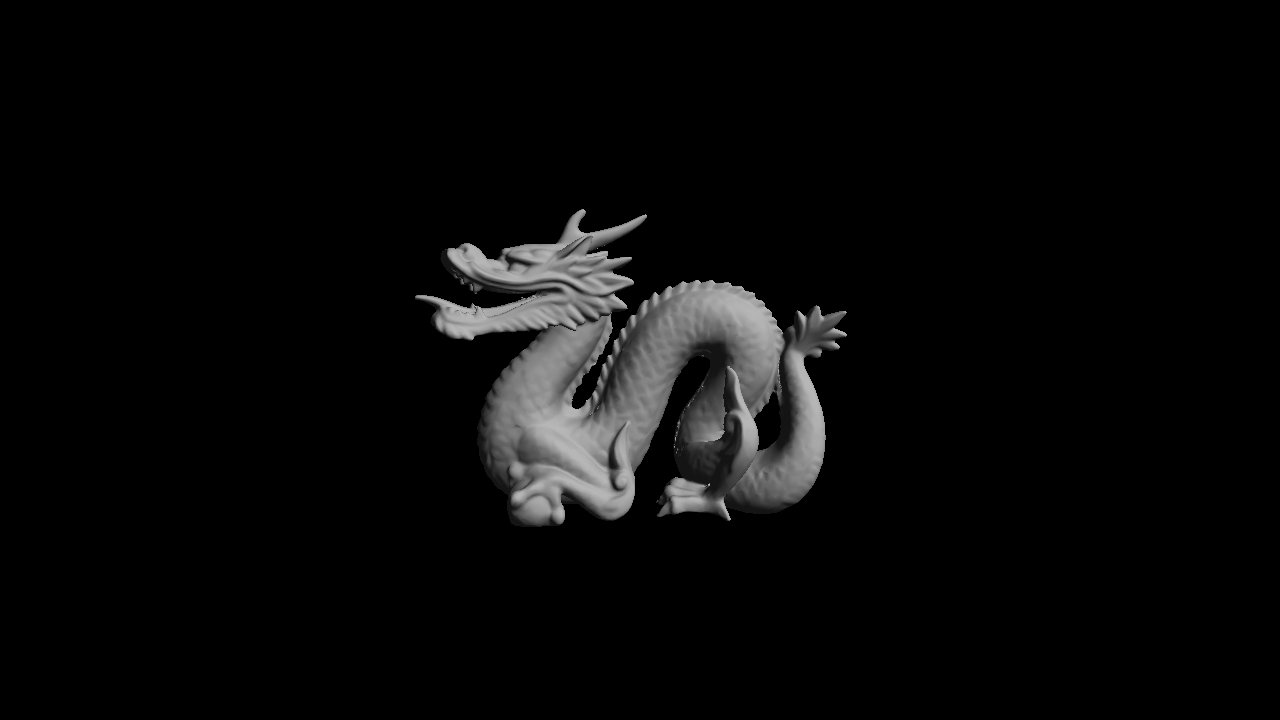
This post will examine the Wavefront OBJ file format and present a preliminary loader in C++. We will overlook the format's support for materials and focus purely on the geometry. Once our model has been loaded, an OpenGL Display List will be used to render the model. Below is a rendering of a dragon model …