The path tracer we will create in this project will run on CUDA-enabled GPUs. You will need to install the CUDA Toolkit available from NVIDIA. The device code for this project uses classes and must be compiled with compute capability 2.0. If you are unsure what compute capability your card has, check out this list.
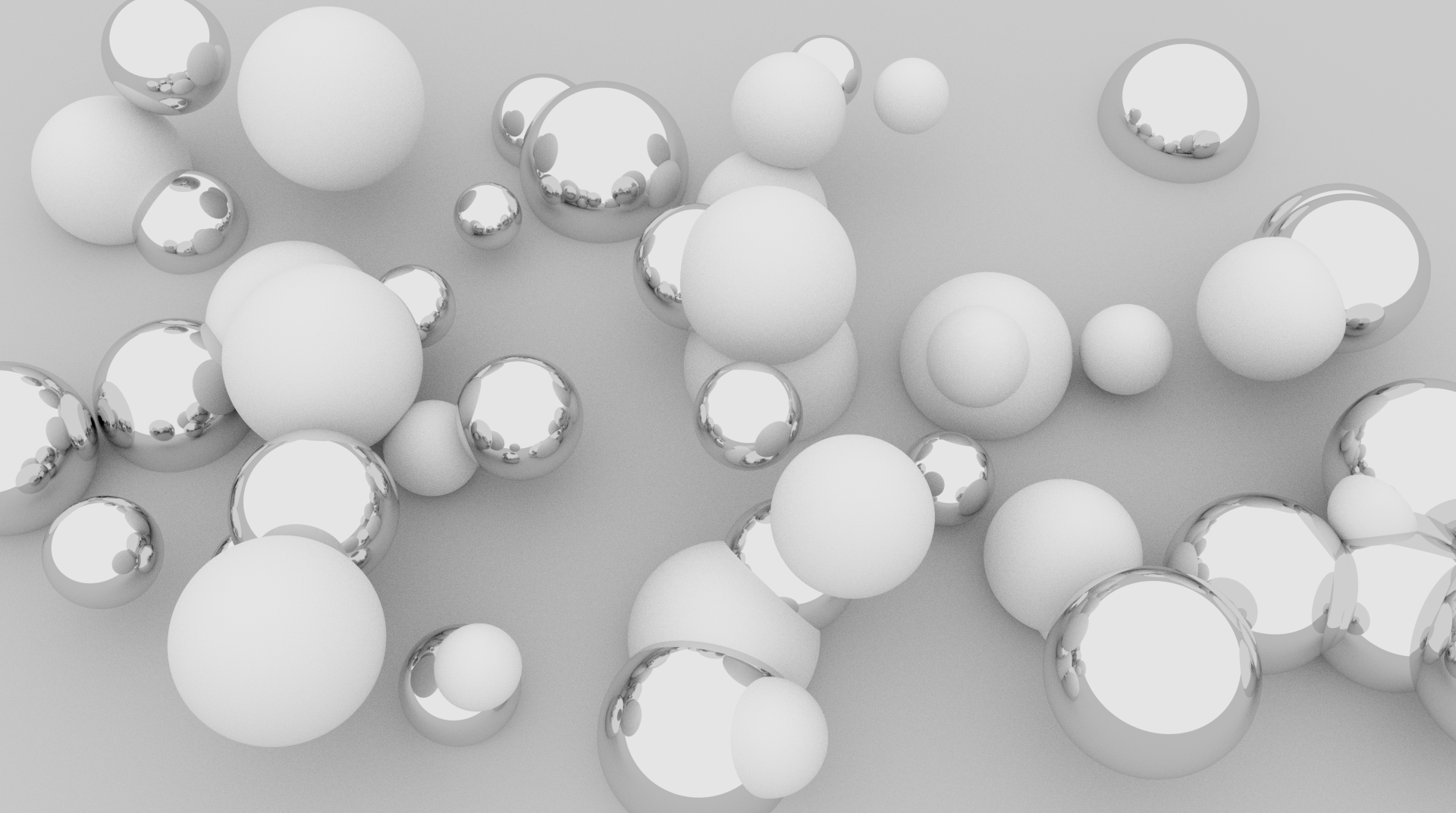
Below are two screen captures of this project in action.


This path tracer is basic and fairly crude and inefficient. I'll provide a brief overview of the code before we delve into some of the mathematics. The host code defines an abstract base class, cObject, from which the cPlane and cSphere objects are derived. The base class includes the material type, color, emission color and type (plane or sphere) properties. The applyCamera() virtual function is defined in the super classes and transforms the respective object into camera space.
The objects in camera space are passed to the device where the environment is rendered. The runPathTracer() function in pathtracer.cu generates some random numbers, executes the kernel, and retrieves the current frame. This frame is rendered to a texture during program execution and saved to a ppm file upon program termination.
The kernel function runs through our buffer, and for each buffer location four rays are shot out in each of the four quadrants surrounding the buffer location using cosine-weighted sampling. These four samples are averaged and added to the accumulation. The device function, sampleRay(), is called on each ray. A maximum loop size is defined (e.g. 5 bounces), and sampling begins for the current ray.
The ray sampler loops over the maximum number of bounces. Within this loop, we loop over our objects seeking an intersection using the equations outlined below for spheres and planes. If an intersection is found (the nearest intersection), we set the values in our emission and color arrays and bounce the ray according to the material type (diffuse, specular, or refractive). Lastly, we apply the emission and color arrays to our final sample. If our final sample is \(\vec{s}_1\) and the emission and color values are \(\vec{e}_n\) and \(\vec{c}_n\), respectively, for \(n \in {1,2,...,m}\), where \(m\) is the bounce limit, the result would be,
\begin{align}
\vec{s}_{m} &= \vec{e}_m\\
\vec{s}_{n} &= \vec{e}_{n} + \vec{c}_{n} \circ \vec{s}_{n+1}\\
\end{align}
Below we will discuss some of the mathematics involved in the process before we mention interaction and conclude with a few notes.
Sphere intersection
Our path tracer will include support for spheres and planes. Below we have the equation for a sphere and a ray followed by the evaluation of the point of intersection, \(\vec{p}\). We have a point of intersection provided the determinant of the quadratic equation is positive. Lastly, we evaluate the surface normal by subtracting the sphere center from the point of intersection. Note that when we evaluate the roots of the quadratic, we will select the lesser of the two roots (the nearest point of intersection).
\begin{align}
(\vec{p} - \vec{c}) \cdot (\vec{p} - \vec{c}) &= r^2\\
\vec{r}(t) &= \vec{o} + \vec{r}t\\
(\vec{o} + \vec{r}t - \vec{c}) \cdot (\vec{o} + \vec{r}t - \vec{c}) &= r^2\\
(\vec{r}\cdot\vec{r})t^2 + 2 \cdot \vec{r} (\vec{o} - \vec{c}) t + (\vec{o} - \vec{c}) \cdot (\vec{o} - \vec{c}) - r^2 &= 0\\
\vec{n} &= \vec{p} - \vec{c}\\
\end{align}
Plane intersection
Below we have the equation for a plane followed by an evaluation of the point of intersection. Note that if the ray is parallel to the plane we have either no intersection or an unlimited number of intersections (the line is in the plane). Here we do not need to evaluate the normal, it is an inherent property of the plane.
\begin{align}
(\vec{p} - \vec{p}_0) \cdot \hat{n} &= 0\\
\vec{r}(t) &= \vec{o} + \vec{r}t\\
(\vec{o} + \vec{r}t - \vec{p}_0) \cdot \vec{n} &= 0\\
\end{align}
Specular reflection
The simplest of the three lighting models we will implement in this project, specular reflection gives objects a mirror-like quality. Incoming rays are reflected off the surface of an object in a direction uniquely defined by the incoming ray, \(\vec{r}\), and the unit vector normal to the surface at the point of intersection, \(\hat{n}\).
\begin{align}
\vec{t} &= 2(\hat{n}\cdot\vec{r})\hat{n} - \vec{r}\\
\end{align}
Diffuse reflection
To implement diffuse reflections we will use cosine-weighted sampling. More information on cosine-weighted sampling can be found here. Below \(u_1\) and \(u_2\) are uniform random variables. Ultimately, we will reorient the resultant vector based on the surface normal (we are sampling from the unit hemisphere defined by the surface normal at the point of intersection).
\begin{align}
u_1 &\sim U(0,1)\\
u_2 &\sim U(0,1)\\
r &= \sqrt{1-u_1}\\
\theta &= 2\pi u_2\\
\vec{v} &=
\begin{pmatrix}
r \cos(\theta)\\
r \sin(\theta)\\
\sqrt{u_1}\\
\end{pmatrix}
\end{align}
Refaction
Refraction gives the appearance of light traveling through a barrier, such as from air to glass. Below we have the equation for the transmission vector, \(\vec{t}\), based on Snell's equations. \(n_1\) and \(n_2\) are the indices of refraction of the two media. Obviously, this equation is only valid if the quantity under the radical is nonnegative. If this quantity is negative, we use the reflection equation above. Such a situation is known as total internal reflection. In our code we will intialize \(n_1\) and \(n_2\) by evaluating the inner product of the ray with the surface normal. If this product is less than zero, we will be entering the medium. We also flip the normal when exiting the medium. It should be relatively straight forward to add the Fresnel equations. Kevin Beason did so here.
\begin{align}
\vec{t} &= \frac{n_1}{n_2}\hat{r} - \left( \frac{n_1}{n_2} \hat{n}\cdot\hat{r} + \sqrt{1-\frac{n_1^2}{n_2^2} \left[1 - (\hat{n} \cdot \hat{r})^2 \right]} \right) \cdot \hat{n}\\
\end{align}
A spice of interaction
We have attempted to add some interaction to this project by including the keyboard handler available here. The premise behind this procedure is to reset the accumulated path values when the camera position or orientation changes. The path tracer begins to progressively refine the scene when the view remains static. Improvements to the project's efficiency would yield a better interactive experience.
Some notes
The larger the surface area of your light sources, the faster your scene will appear to converge (less noise), because the rays will hit a light source with greater probability. The project currently has a limit of 10 bounces. If you wish to exceed this limit, you must update the sampleRay() function in pathtracer.cu. Additionally, you will need to update the Makefile to reference the proper location for the libcudart.so and libcurand.so libraries.
If you have any suggestions for improving this path tracer or questions about it, let me know.
Download this project: pathtracer.tar.bz2
Additional information: