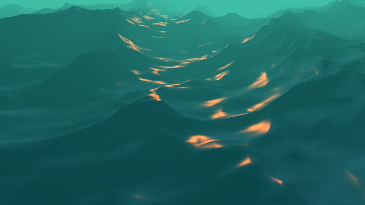
In this post we will implement the statistical wave model from the equations in Tessendorf's paper[1] on simulating ocean water. We will implement this model using a discrete Fourier transform. In part two we will begin with the same equations but provide a deeper analysis in order to implement our own fast Fourier transform. Using the fast Fourier transform, we will be able to achieve interactive frame rates. Below are two screen captures. The first is a rendering of the surface using some of the features from the post on lighting with GLSL with the addition of a simple fog factor. The second is a rendering of the surface mesh.


We begin with the equation for the wave height \(h(\vec{x},t)\) at a location, \(\vec{x} = (x,z)\), and time, \(t\),
\begin{align*}
h(\vec{x},t) &= \sum_\vec{k} \tilde{h}(\vec{k},t)\exp(i\vec{k}\cdot\vec{x})
\end{align*}
We define \(\vec{k}=(k_x,k_z)\) as,
\begin{align*}
k_x &= \frac{2\pi n}{L_x}\\
k_z &= \frac{2\pi m}{L_z}\\
\end{align*}
where,
\begin{align*}
-\frac{N}{2} \le &n < \frac{N}{2} \\
-\frac{M}{2} \le &m < \frac{M}{2} \\
\end{align*}
In our implementation our indices, \(n'\) and \(m'\), will run from \(0,1,...,N-1\) and \(0,1,...,M-1\), respectively. So we have,
\begin{align*}
0 \le &n' < N\\
0 \le &m' < M\\
\end{align*}
Thus, \(n\) and \(m\) can be written in terms of \(n'\) and \(m'\),
\begin{align*}
n &= n'-\frac{N}{2}\\
m &= m'-\frac{M}{2}\\
\end{align*}
\(\vec{k}\) in terms of \(n'\) and \(m'\),
\begin{align*}
k_x &= \frac{2\pi (n'-\frac{N}{2})}{L_x}\\
&= \frac{2\pi n'- \pi N}{L_x}\\
k_z &= \frac{2\pi (m'-\frac{M}{2})}{L_z}\\
&= \frac{2\pi m'- \pi M}{L_z}\\
\end{align*}
We can now write our original equation for the wave height in terms of \(n'\) and \(m'\) as,
\begin{align*}
h'(x,z,t) &= \sum_{m'=0}^{M-1} \sum_{n'=0}^{N-1} \tilde{h}'(n',m',t)\exp\left(\frac{ix(2\pi n' - \pi N)}{L_x} + \frac{iz(2\pi m' - \pi M)}{L_z}\right)
\end{align*}
We still need to look at the function, \(\tilde{h}\), as a function of \(\vec{k}\) and \(t\) and our equivalent function, \(\tilde{h}'\), as a function of our indices, \(n'\) and \(m'\), and \(t\). \(\tilde{h}(\vec{k},t)\) is defined as,
\begin{align*}
\tilde{h}(\vec{k},t) = &\tilde{h}_0(\vec{k}) \exp(i\omega(k)t) +\\ &\tilde{h}_0^*(-\vec{k})\exp(-i\omega(k)t) \\
\tilde{h}'(n',m',t) = &\tilde{h}_0'(n',m') \exp(i\omega'(n',m')t) +\\ &{\tilde{h}_0'}^*(-n',-m')\exp(-i\omega'(n',m')t) \\
\end{align*}
where \(\omega(k)\) is the dispersion relation given by,
\begin{align*}
\omega(k) = \sqrt{gk} \\
\end{align*}
and \(g\) is the local acceleration due to gravity, nominally \(9.8\frac{m}{\sec^2}\). In terms of our indices,
\begin{align*}
\omega'(n',m') = \sqrt{g\sqrt{\left(\frac{2\pi n'- \pi N}{L_x}\right)^2+\left(\frac{2\pi m'- \pi M}{L_z}\right)^2}} \\
\end{align*}
We are almost there, but we need \(\tilde{h}_0'\) and the complex conjugate, \({\tilde{h}_0'}^*\), in terms of our indices,
\begin{align*}
\tilde{h}_0(\vec{k}) &= \frac{1}{\sqrt{2}}(\xi_r+i\xi{i})\sqrt{P_h(\vec{k})} \\
\tilde{h}_0'(n',m') &= \frac{1}{\sqrt{2}}(\xi_r+i\xi{i})\sqrt{P_h'(n',m')} \\
\end{align*}
where \(\xi_r\) and \(\xi_i\) are independent gaussian random variables. \(P_h(\vec{k})\) is the Phillips spectrum given by,
\begin{align*}
P_h(\vec{k}) &= A\frac{\exp(-1/(kL)^2)}{k^4}|\vec{k}\cdot \vec{w}|^2 \\
\end{align*}
where \(\vec{w}\) is the direction of the wind and \(L=V^2/g\) is the largest possible waves arising from a continuous wind of speed \(V\). In terms of the indices,
\begin{align*}
P_h'(n',m') &= A\frac{\exp(-1/(kL)^2)}{k^4}|\vec{k}\cdot \vec{w}|^2 \\
\vec{k} &= \left(\frac{2\pi n'- \pi N}{L_x}, \frac{2\pi m'- \pi M}{L_z}\right) \\
k &= |\vec{k}| \\
\end{align*}
We should now have everything we need to render our wave height field, but we will evaluate a displacement vector for generating choppy waves and the normal vector for our lighting calculations at each vertex. The displacement vector is given by,
\begin{align*}
\vec{D}(\vec{x},t) &= \sum_{\vec{k}}-i\frac{\vec{k}}{k}\tilde{h}(\vec{k},t)\exp(i\vec{k}\cdot \vec{x}) \\
\end{align*}
and the normal vector, \(\vec{N}\), is given by,
\begin{align*}
\epsilon(\vec{x},t) &= \nabla h(\vec{x},t) = \sum_{\vec{k}}i\vec{k}\tilde{h}(\vec{k},t)\exp(i\vec{k}\cdot \vec{x}) \\
\vec{N}(\vec{x},t) &= (0,1,0) - \left(\epsilon_x(\vec{x},t), 0, \epsilon_z(\vec{x},t)\right) \\
&= \left(-\epsilon_x(\vec{x},t), 1, -\epsilon_z(\vec{x},t)\right) \\
\end{align*}
all of which we can rewrite in terms of the indices for ease of implementation. We'll begin our implementation by looking at our vertex structure which will double to hold our values for \(\tilde{h}_0'(n',m')\) and \({\tilde{h}_0'}^*(-n',-m')\). We will apply our wave height and displacement vector to ox, oy, and oz to obtain the current position, x, y, and z.
struct vertex_ocean {
	GLfloat   x,   y,   z; // vertex
	GLfloat  nx,  ny,  nz; // normal
	GLfloat   a,   b,   c; // htilde0
	GLfloat  _a,  _b,  _c; // htilde0mk conjugate
	GLfloat  ox,  oy,  oz; // original position
};
We have another structure to return the resulting wave height, displacement vector, and normal vector at a location, \(\vec{x}\), and time, \(t\),
struct complex_vector_normal {	// structure used with discrete fourier transform
	complex h;		// wave height
	vector2 D;		// displacement
	vector3 n;		// normal
};
The following is the declaration of our cOcean object. There are references to the fast Fourier transform which we will cover in the next post. In this implementation we are assuming \(M=N\) and \(L=L_x=L_z\) from the equations above. We declare the property, Nplus1, for tiling purposes in order for our vertices to connect to the tile at an adjacent location.
class cOcean {
  private:
	bool geometry;							// flag to render geometry or surface

	float g;								// gravity constant
	int N, Nplus1;							// dimension -- N should be a power of 2
	float A;								// phillips spectrum parameter -- affects heights of waves
	vector2 w;								// wind parameter
	float length;							// length parameter
	complex *h_tilde,						// for fast fourier transform
		*h_tilde_slopex, *h_tilde_slopez,
		*h_tilde_dx, *h_tilde_dz;
	cFFT *fft;								// fast fourier transform

	vertex_ocean *vertices;					// vertices for vertex buffer object
	unsigned int *indices;					// indicies for vertex buffer object
	unsigned int indices_count;				// number of indices to render
	GLuint vbo_vertices, vbo_indices;		// vertex buffer objects

	GLuint glProgram, glShaderV, glShaderF;	// shaders
	GLint vertex, normal, texture, light_position, projection, view, model;	// attributes and uniforms

  protected:
  public:
	cOcean(const int N, const float A, const vector2 w, const float length, bool geometry);
	~cOcean();
	void release();

	float dispersion(int n_prime, int m_prime);		// deep water
	float phillips(int n_prime, int m_prime);		// phillips spectrum
	complex hTilde_0(int n_prime, int m_prime);
	complex hTilde(float t, int n_prime, int m_prime);
	complex_vector_normal h_D_and_n(vector2 x, float t);
	void evaluateWaves(float t);
	void evaluateWavesFFT(float t);
	void render(float t, glm::vec3 light_pos, glm::mat4 Projection, glm::mat4 View, glm::mat4 Model, bool use_fft);
};
In our constructor we set up some resources, define our vertices and indices for the vertex buffer objects, create our shader program, and, lastly, generate our vertex buffer objects. The destructor frees our resources, and the release method frees our vertex buffer objects and shader program before our OpenGL context is destroyed.
cOcean::cOcean(const int N, const float A, const vector2 w, const float length, const bool geometry) :
	g(9.81), geometry(geometry), N(N), Nplus1(N+1), A(A), w(w), length(length),
	vertices(0), indices(0), h_tilde(0), h_tilde_slopex(0), h_tilde_slopez(0), h_tilde_dx(0), h_tilde_dz(0), fft(0)
{
	h_tilde        = new complex[N*N];
	h_tilde_slopex = new complex[N*N];
	h_tilde_slopez = new complex[N*N];
	h_tilde_dx     = new complex[N*N];
	h_tilde_dz     = new complex[N*N];
	fft            = new cFFT(N);
	vertices       = new vertex_ocean[Nplus1*Nplus1];
	indices        = new unsigned int[Nplus1*Nplus1*10];

	int index;

	complex htilde0, htilde0mk_conj;
	for (int m_prime = 0; m_prime < Nplus1; m_prime++) {
		for (int n_prime = 0; n_prime < Nplus1; n_prime++) {
			index = m_prime * Nplus1 + n_prime;

			htilde0        = hTilde_0( n_prime,  m_prime);
			htilde0mk_conj = hTilde_0(-n_prime, -m_prime).conj();

			vertices[index].a  = htilde0.a;
			vertices[index].b  = htilde0.b;
			vertices[index]._a = htilde0mk_conj.a;
			vertices[index]._b = htilde0mk_conj.b;

			vertices[index].ox = vertices[index].x =  (n_prime - N / 2.0f) * length / N;
			vertices[index].oy = vertices[index].y =  0.0f;
			vertices[index].oz = vertices[index].z =  (m_prime - N / 2.0f) * length / N;

			vertices[index].nx = 0.0f;
			vertices[index].ny = 1.0f;
			vertices[index].nz = 0.0f;
		}
	}

	indices_count = 0;
	for (int m_prime = 0; m_prime < N; m_prime++) {
		for (int n_prime = 0; n_prime < N; n_prime++) {
			index = m_prime * Nplus1 + n_prime;

			if (geometry) {
				indices[indices_count++] = index;				// lines
				indices[indices_count++] = index + 1;
				indices[indices_count++] = index;
				indices[indices_count++] = index + Nplus1;
				indices[indices_count++] = index;
				indices[indices_count++] = index + Nplus1 + 1;
				if (n_prime == N - 1) {
					indices[indices_count++] = index + 1;
					indices[indices_count++] = index + Nplus1 + 1;
				}
				if (m_prime == N - 1) {
					indices[indices_count++] = index + Nplus1;
					indices[indices_count++] = index + Nplus1 + 1;
				}
			} else {
				indices[indices_count++] = index;				// two triangles
				indices[indices_count++] = index + Nplus1;
				indices[indices_count++] = index + Nplus1 + 1;
				indices[indices_count++] = index;
				indices[indices_count++] = index + Nplus1 + 1;
				indices[indices_count++] = index + 1;
			}
		}
	}

	createProgram(glProgram, glShaderV, glShaderF, "src/oceanv.sh", "src/oceanf.sh");
	vertex         = glGetAttribLocation(glProgram, "vertex");
	normal         = glGetAttribLocation(glProgram, "normal");
	texture        = glGetAttribLocation(glProgram, "texture");
	light_position = glGetUniformLocation(glProgram, "light_position");
	projection     = glGetUniformLocation(glProgram, "Projection");
	view           = glGetUniformLocation(glProgram, "View");
	model          = glGetUniformLocation(glProgram, "Model");

	glGenBuffers(1, &vbo_vertices);
	glBindBuffer(GL_ARRAY_BUFFER, vbo_vertices);
	glBufferData(GL_ARRAY_BUFFER, sizeof(vertex_ocean)*(Nplus1)*(Nplus1), vertices, GL_DYNAMIC_DRAW);

	glGenBuffers(1, &vbo_indices);
	glBindBuffer(GL_ELEMENT_ARRAY_BUFFER, vbo_indices);
	glBufferData(GL_ELEMENT_ARRAY_BUFFER, indices_count*sizeof(unsigned int), indices, GL_STATIC_DRAW);
}

cOcean::~cOcean() {
	if (h_tilde)		delete [] h_tilde;
	if (h_tilde_slopex)	delete [] h_tilde_slopex;
	if (h_tilde_slopez)	delete [] h_tilde_slopez;
	if (h_tilde_dx)		delete [] h_tilde_dx;
	if (h_tilde_dz)		delete [] h_tilde_dz;
	if (fft)		delete fft;
	if (vertices)		delete [] vertices;
	if (indices)		delete [] indices;
}

void cOcean::release() {
	glDeleteBuffers(1, &vbo_indices);
	glDeleteBuffers(1, &vbo_vertices);
	releaseProgram(glProgram, glShaderV, glShaderF);
}
Below are our helper methods for evaluating the disperson relation and the Phillips spectrum in addition to \(\tilde{h}_0'\) and \(\tilde{h}'\).
float cOcean::dispersion(int n_prime, int m_prime) {
	float w_0 = 2.0f * M_PI / 200.0f;
	float kx = M_PI * (2 * n_prime - N) / length;
	float kz = M_PI * (2 * m_prime - N) / length;
	return floor(sqrt(g * sqrt(kx * kx + kz * kz)) / w_0) * w_0;
}

float cOcean::phillips(int n_prime, int m_prime) {
	vector2 k(M_PI * (2 * n_prime - N) / length,
		  M_PI * (2 * m_prime - N) / length);
	float k_length  = k.length();
	if (k_length < 0.000001) return 0.0;

	float k_length2 = k_length  * k_length;
	float k_length4 = k_length2 * k_length2;

	float k_dot_w   = k.unit() * w.unit();
	float k_dot_w2  = k_dot_w * k_dot_w;

	float w_length  = w.length();
	float L         = w_length * w_length / g;
	float L2        = L * L;

	float damping   = 0.001;
	float l2        = L2 * damping * damping;

	return A * exp(-1.0f / (k_length2 * L2)) / k_length4 * k_dot_w2 * exp(-k_length2 * l2);
}

complex cOcean::hTilde_0(int n_prime, int m_prime) {
	complex r = gaussianRandomVariable();
	return r * sqrt(phillips(n_prime, m_prime) / 2.0f);
}

complex cOcean::hTilde(float t, int n_prime, int m_prime) {
	int index = m_prime * Nplus1 + n_prime;

	complex htilde0(vertices[index].a,  vertices[index].b);
	complex htilde0mkconj(vertices[index]._a, vertices[index]._b);

	float omegat = dispersion(n_prime, m_prime) * t;

	float cos_ = cos(omegat);
	float sin_ = sin(omegat);

	complex c0(cos_,  sin_);
	complex c1(cos_, -sin_);

	complex res = htilde0 * c0 + htilde0mkconj * c1;

	return htilde0 * c0 + htilde0mkconj*c1;
}
We have the method, h_D_and_n, to evaluate the wave height, displacement vector, and normal vector at a location, \(\vec{x}\).
complex_vector_normal cOcean::h_D_and_n(vector2 x, float t) {
	complex h(0.0f, 0.0f);
	vector2 D(0.0f, 0.0f);
	vector3 n(0.0f, 0.0f, 0.0f);

	complex c, res, htilde_c;
	vector2 k;
	float kx, kz, k_length, k_dot_x;

	for (int m_prime = 0; m_prime < N; m_prime++) {
		kz = 2.0f * M_PI * (m_prime - N / 2.0f) / length;
		for (int n_prime = 0; n_prime < N; n_prime++) {
			kx = 2.0f * M_PI * (n_prime - N / 2.0f) / length;
			k = vector2(kx, kz);

			k_length = k.length();
			k_dot_x = k * x;

			c = complex(cos(k_dot_x), sin(k_dot_x));
			htilde_c = hTilde(t, n_prime, m_prime) * c;

			h = h + htilde_c;

			n = n + vector3(-kx * htilde_c.b, 0.0f, -kz * htilde_c.b);

			if (k_length < 0.000001) continue;
			D = D + vector2(kx / k_length * htilde_c.b, kz / k_length * htilde_c.b);
		}
	}

	n = (vector3(0.0f, 1.0f, 0.0f) - n).unit();

	complex_vector_normal cvn;
	cvn.h = h;
	cvn.D = D;
	cvn.n = n;
	return cvn;
}
Below we have a method to evaluate our waves using the h_D_and_n method. Note the tiling under the conditions, \(n'=m'=0\), \(n'=0\), and \(m'=0\).
void cOcean::evaluateWaves(float t) {
	float lambda = -1.0;
	int index;
	vector2 x;
	vector2 d;
	complex_vector_normal h_d_and_n;
	for (int m_prime = 0; m_prime < N; m_prime++) {
		for (int n_prime = 0; n_prime < N; n_prime++) {
			index = m_prime * Nplus1 + n_prime;

			x = vector2(vertices[index].x, vertices[index].z);

			h_d_and_n = h_D_and_n(x, t);

			vertices[index].y = h_d_and_n.h.a;

			vertices[index].x = vertices[index].ox + lambda*h_d_and_n.D.x;
			vertices[index].z = vertices[index].oz + lambda*h_d_and_n.D.y;

			vertices[index].nx = h_d_and_n.n.x;
			vertices[index].ny = h_d_and_n.n.y;
			vertices[index].nz = h_d_and_n.n.z;

			if (n_prime == 0 && m_prime == 0) {
				vertices[index + N + Nplus1 * N].y = h_d_and_n.h.a;

				vertices[index + N + Nplus1 * N].x = vertices[index + N + Nplus1 * N].ox + lambda*h_d_and_n.D.x;
				vertices[index + N + Nplus1 * N].z = vertices[index + N + Nplus1 * N].oz + lambda*h_d_and_n.D.y;

				vertices[index + N + Nplus1 * N].nx = h_d_and_n.n.x;
				vertices[index + N + Nplus1 * N].ny = h_d_and_n.n.y;
				vertices[index + N + Nplus1 * N].nz = h_d_and_n.n.z;
			}
			if (n_prime == 0) {
				vertices[index + N].y = h_d_and_n.h.a;

				vertices[index + N].x = vertices[index + N].ox + lambda*h_d_and_n.D.x;
				vertices[index + N].z = vertices[index + N].oz + lambda*h_d_and_n.D.y;

				vertices[index + N].nx = h_d_and_n.n.x;
				vertices[index + N].ny = h_d_and_n.n.y;
				vertices[index + N].nz = h_d_and_n.n.z;
			}
			if (m_prime == 0) {
				vertices[index + Nplus1 * N].y = h_d_and_n.h.a;

				vertices[index + Nplus1 * N].x = vertices[index + Nplus1 * N].ox + lambda*h_d_and_n.D.x;
				vertices[index + Nplus1 * N].z = vertices[index + Nplus1 * N].oz + lambda*h_d_and_n.D.y;

				vertices[index + Nplus1 * N].nx = h_d_and_n.n.x;
				vertices[index + Nplus1 * N].ny = h_d_and_n.n.y;
				vertices[index + Nplus1 * N].nz = h_d_and_n.n.z;
			}
		}
	}
}
Finally, we have our render method. We have a static variable, eval. Under the condition that we are not using the fast Fourier transform, we simply update our vertices and normals during the first frame. This will permit us to navigate the first frame of our wave height field in our main function. We then specify the uniforms and attribute offsets for our shader program and then render either the surface or the geometry.
void cOcean::render(float t, glm::vec3 light_pos, glm::mat4 Projection, glm::mat4 View, glm::mat4 Model, bool use_fft) {
	static bool eval = false;
	if (!use_fft && !eval) {
		eval = true;
		evaluateWaves(t);
	} else if (use_fft) {
		evaluateWavesFFT(t);
	}

	glUseProgram(glProgram);
	glUniform3f(light_position, light_pos.x, light_pos.y, light_pos.z);
	glUniformMatrix4fv(projection, 1, GL_FALSE, glm::value_ptr(Projection));
	glUniformMatrix4fv(view,       1, GL_FALSE, glm::value_ptr(View));
	glUniformMatrix4fv(model,      1, GL_FALSE, glm::value_ptr(Model));

	glBindBuffer(GL_ARRAY_BUFFER, vbo_vertices);
	glBufferSubData(GL_ARRAY_BUFFER, 0, sizeof(vertex_ocean) * Nplus1 * Nplus1, vertices);
	glEnableVertexAttribArray(vertex);
	glVertexAttribPointer(vertex, 3, GL_FLOAT, GL_FALSE, sizeof(vertex_ocean), 0);
	glEnableVertexAttribArray(normal);
	glVertexAttribPointer(normal, 3, GL_FLOAT, GL_FALSE, sizeof(vertex_ocean), (char *)NULL + 12);
	glEnableVertexAttribArray(texture);
	glVertexAttribPointer(texture, 3, GL_FLOAT, GL_FALSE, sizeof(vertex_ocean), (char *)NULL + 24);

	glBindBuffer(GL_ELEMENT_ARRAY_BUFFER, vbo_indices);
	for (int j = 0; j < 10; j++) {
		for (int i = 0; i < 10; i++) {
			Model = glm::scale(glm::mat4(1.0f), glm::vec3(5.f, 5.f, 5.f));
			Model = glm::translate(Model, glm::vec3(length * i, 0, length * -j));
			glUniformMatrix4fv(model, 1, GL_FALSE, glm::value_ptr(Model));
			glDrawElements(geometry ? GL_LINES : GL_TRIANGLES, indices_count, GL_UNSIGNED_INT, 0);
		}
	}
}
In the code above there are references to the complex, vector2, and vector3 objects. These are available in the download. Any library that supports complex variables in addition to 2-dimensional and 3-dimensional vectors would be appropriate. Additionally, we have used Euler's formula in our code above. Euler's formula states for any real \(x\),
\begin{align*}
\exp(ix) &= \cos x + i\sin x \\
\end{align*}
This post is simply a brute force evaluation of our ocean surface using the discrete Fourier transform. In the following post we will provide a deeper analysis of the equations used here to implement our own fast Fourier transform algorithm. The download for this project includes a fast Fourier transform, so have a look at it and we'll analyze it in the next post.
I've added a mouse handler in a vain similar to the keyboard handler and joystick handler from previous posts. The source code expects the keyboard device node to be located at /dev/input/event0 and the device node for the mouse to be located at /dev/input/event1. You can navigate using the mouse and the WASD keys.
One last thing to mention is in regards to the fog factor. Below is the vertex shader which is reminiscent of our previous shaders with the addition of the fog_factor variable. We simply divide the z coordinate of our vertex position in view space to retrieve a fog factor in the interval \([0,1]\).
#version 330

in vec3 vertex;
in vec3 normal;
in vec3 texture;

uniform mat4 Projection;
uniform mat4 View;
uniform mat4 Model;
uniform vec3 light_position;

out vec3 light_vector;
out vec3 normal_vector;
out vec3 halfway_vector;
out float fog_factor;
out vec2 tex_coord;

void main() {
	gl_Position = View * Model * vec4(vertex, 1.0);
	fog_factor = min(-gl_Position.z/500.0, 1.0);
	gl_Position = Projection * gl_Position;

	vec4 v = View * Model * vec4(vertex, 1.0);
	vec3 normal1 = normalize(normal);

	light_vector = normalize((View * vec4(light_position, 1.0)).xyz - v.xyz);
	normal_vector = (inverse(transpose(View * Model)) * vec4(normal1, 0.0)).xyz;
        halfway_vector = light_vector + normalize(-v.xyz);

	tex_coord = texture.xy;
}
In the fragment shader we simply apply the fog factor to the final fragment color.
#version 330

in vec3 normal_vector;
in vec3 light_vector;
in vec3 halfway_vector;
in vec2 tex_coord;
in float fog_factor;
uniform sampler2D water;
out vec4 fragColor;

void main (void) {
	//fragColor = vec4(1.0, 1.0, 1.0, 1.0);

	vec3 normal1         = normalize(normal_vector);
	vec3 light_vector1   = normalize(light_vector);
	vec3 halfway_vector1 = normalize(halfway_vector);

	vec4 c = vec4(1,1,1,1);//texture(water, tex_coord);

	vec4 emissive_color = vec4(1.0, 1.0, 1.0,  1.0);
	vec4 ambient_color  = vec4(0.0, 0.65, 0.75, 1.0);
	vec4 diffuse_color  = vec4(0.5, 0.65, 0.75, 1.0);
	vec4 specular_color = vec4(1.0, 0.25, 0.0,  1.0);

	float emissive_contribution = 0.00;
	float ambient_contribution  = 0.30;
	float diffuse_contribution  = 0.30;
	float specular_contribution = 1.80;

	float d = dot(normal1, light_vector1);
	bool facing = d > 0.0;

	fragColor = emissive_color * emissive_contribution +
		    ambient_color  * ambient_contribution  * c +
		    diffuse_color  * diffuse_contribution  * c * max(d, 0) +
                    (facing ?
			specular_color * specular_contribution * c * max(pow(dot(normal1, halfway_vector1), 120.0), 0.0) :
			vec4(0.0, 0.0, 0.0, 0.0));

	fragColor = fragColor * (1.0-fog_factor) + vec4(0.25, 0.75, 0.65, 1.0) * (fog_factor);

	fragColor.a = 1.0;
}
If you have any questions or comments, let me know. We will continue with this project in the next post.
Download this project: waves.dft_correction20121002.tar.bz2
References:
1. Tessendorf, Jerry. Simulating Ocean Water. In SIGGRAPH 2002 Course Notes #9 (Simulating Nature: Realistic and Interactive Techniques), ACM Press.

Comments
Keith,
I am impressed with your ocean simulations.
I am looking for paid help to use/adopt your formulation/code in Unity3d.
If interested and available, please let me know.
Thanks,
DA
Author
Hey Dan,
That sounds like an interesting project, but I don't think I'll find the time to work on it.
Help yourself to the code, though. If you can find a place to use it, go for it.
Keith
Your conjugate method is missing something?
Shouldn't
complex complex::conj() { return complex(this->a, this->b); }
be
complex complex::conj() { return complex(this->a, -this->b); }
?
Author
Hey Håvard..
Good eye.. I've updated the code for this project and the one on using the fft.
Thanks.
Pingback: 3ds max Lab sandbox examples. « Håvard Schei
Where can I learn the math required to understand this? Thanks. I'm eager to try this out!
Author
Is there a particular section you are stuck on?
I just don't understand the equation for wave height.
Author
Hey.. I'm not sure what kind of background you have, but you may start with some research on the Fourier transform. Also, looking through the code and seeing how that correlates with the derivation might help. If you have a specific question, it might be easier for me to suggest a direction for you.
Hi
Thank you for a great tutorial.
I´m still puzzled about the tiling part with the last three "if statements"
what are they for exactly ?
Author
Hey David,
Because we can tile this seamlessly, we've defined the size of the grid as
Nplus1. When we evaluate the wave heights, we only evaluate those heights on the N by N grid. The last row and column are reserved to equal the wave heights of the first row and column, respectively. If we were dealing only with points, we wouldn't need this extra row and column, but we want to fill that row and column with primitives, so those vertices have been added to draw the triangles. The first corner is a special case for adding the primitives to the last corner.Since the height of the last vertices match those of the first, we can fit the second tile next to the first, and it will appear seamless.
I see ... thank you !
first Thanks for your post .
i compile it under windows but the code
createProgram(glProgram, glShaderV, glShaderF, "src/oceanv.sh", "src/oceanf.sh") is wrong
there is no this func would you tell how can i deal with it? sorry for my poor english
Author
Hey..
The
createProgram()function is defined insrc/glhelper.cc. That source file is compiled and placed inlib/glhelper.o. This object file should be linked as the final part of the build process.It should all be there. Do you have any output from the
makeprocess?Thansk a lot for your replay . With the src/glhelper.cc ,the problem above is resolved。
But because I compile it in windows ,so the project miss a lot of header files 。then I install the ubuntu, and it sucessful compiled under ubuntu 。but my notebook compter don‘t have the independent video card,so when i run the main, the consequence is just a black frame 。Is it correct?
Author
That could be.. there isn't a lot of error checking. The shaders,
src/oceanv.shandsrc/oceanf.sh, were written for GLSL v3.3. ThecreateProgram()function might be spitting out the info logs.thanks for your replay but i still can't execute it,maybe i should buy a new computer.
now I have another question and I would appreciate if you can give me some advices.
first ,the simulation of the sea surface is composed of many small triangles ,now I number the triangles from 1 to N*N (the amount of triangle is N*N),then irradiating the sea ,if the angle of incidence of the light is very large,then some triangles will be blocked by others, now my question is how to know which triangles is blocked and output the number of the blocked triangles
Author
Hey..
I think the number of triangles should be \(2 \cdot N \cdot N\). The number of quads would be \(N \cdot N\). My first thought would be to cast a ray from each point on a triangle towards your light source and see if they intersect any other object on the way there, but that would only work if all three points intersect the same triangle on the way to the light source. You might look into shadow casting. That might give you what you're looking for.
thanks for your post
after i compile and execute it ,it shows
error C0000: syntax error, unexpected $end at token ""
(0) : error C0501: type name expected at token ""
(1) : error C0000: syntax error, unexpected $undefined at token ""
(1) : error C0501: type name expected at token ""
(1) : error C1038: declaration of "E" conflicts with previous declaration at (1)
Vertex info
-----------
(0) : error C0000: syntax error, unexpected $end at token ""
(0) : error C0501: type name expected at token ""
Fragment info
-------------
(1) : error C0000: syntax error, unexpected $undefined at token ""
(1) : error C0501: type name expected at token ""
(1) : error C1038: declaration of "E" conflicts with previous declaration at (1)
Author
Hey Jon..
What graphics card do you have? Have you checked if there is a latest driver for your card?
i install a new graphics card gtx650 and it still occurs error like
error C0000: syntax error, unexpected $end at token ""
(0) : error C0501: type name expected at token ""
(1) : error C0000: syntax error, unexpected $undefined at token ""
(1) : error C0501: type name expected at token ""
(1) : error C1038: declaration of "E" conflicts with previous declaration at (1)
Vertex info
-----------
(0) : error C0000: syntax error, unexpected $end at token ""
(0) : error C0501: type name expected at token ""
Fragment info
-------------
(1) : error C0000: syntax error, unexpected $undefined at token ""
(1) : error C0501: type name expected at token ""
(1) : error C1038: declaration of "E" conflicts with previous declaration at (1)
and i feel like breaking down
another question,if i make it in wiondows,where should i rewrite sorry for my english
and thanks for your all replay
thanks a lot. I successfully compiled it and it runs OK in windows
Hi, good article!
I have a question: i adjust Length to 32;
hTilde_0 always return 0, why?
Thanks!
Author
Hey Ferdin..
I apologize for the delay. I've tried changing the
lengthto 32, and it appears to evaluate properly on my side. Are you still having issues with the length?Fantastic article, are you able to explain more on how the displacement vector and the normal vector are derived?
Another question is on the conjugate of the value returned by the function: h'_0(-n',-m',t), shouldn't that function be without the t variable?
Author
Hey Wallace..
You are correct. The equation for \({\tilde{h}_0'}^*\) should be independent of \(t\). I've fixed this. It's been a while since I've worked with this project, so let me get back to you on your first question.
Hi Keith,
I was just wondering if the random numbers Zi and Zr are generated on every frame to calculate h(x,t)? I am doing a similar project and my waves are very jumpy at every frame!
Sen
Author
Hey Sen,
If I recall, the random numbers are generated once to evaluate \(\tilde{h}_0\).
Hi Keith,
Thanks so much for the reply! I must have misunderstood that part - I'll try and fix it with your advice in mind.
Thanks
P.s. I forgot to mention, great tutorial!
Hi Keith,
I did mis-interpret the equation, now the random jumpy-ness has stopped! Thanks!
I still had a couple of small questions if thats ok:
1. When we work out h(x,t) = sum_over_k( h(k,t)*exp(ik.x) ), we are supposed to get a real number for the height - but the the equation for "choppiness" is almost identical to this one, only its multiplied by i*(k/k_magnitude) - surely this will yield a complex number multiplying a vector - how do we interpret this complex number for the shift in (x,z)? Or am i going wrong again!
2. what library are you using to deal with complex numbers? I will be using the "FFTW" library - which would you recommend?
Thanks again!
Author
Hey Sen..
1. You're right.. it will be a complex number. I just took the real part of that number and applied it to the displacement. See the
h_D_and_n()whereDis evaluated. It looks like, technically, I missed a multiplication by \(-1\). However, that seems to be corrected in theevaluateWaves()method by lettinglambda = -1.0.2. I wrote a simple object to deal with complex numbers. In the second part of this project I implemented a FFT to use that complex number object. Beyond that, I'm not very familiar with libraries that implement a FFT. It looks like the FFTW library you mentioned would be a good choice.
hey i was just wondering if you could explain what a complex or send me into the right direction to researching it is I've tried googleing it but all i get are complex shapes also in the hTilde formula you have sin and cos but i cant see them in the equation can you explain why they're in there? cheers
Author
Hey Connor..
Here are a couple of links for you..
http://en.wikipedia.org/wiki/Complex_number
http://en.wikipedia.org/wiki/Euler%27s_formula
thanks you are a huge help. didn't know why i just didn't just look on Wikipedia 😛
hey i was also wondering in h_D_and_n why do you cos and sin k_dot_x? i am following your tutorial writing this all from scratch so i understand it more and so far Ive had no to little trouble. but i couldn't figure out why you did that
hope to hear from you soon 🙂
Author
Hey Connor..
The cos and sin come from Euler's formula:
http://en.wikipedia.org/wiki/Euler%27s_formula
It is being applied to this part of the wave height equation:
\(\exp(i\vec{k}\cdot\vec{x})\)
Dear Keith,
Would have a version of this simulator where you take account, for example, a wave directional spectrum and the resulting image is in gray levels?
André.
Author
Hey André..
I haven't done much with this simulation beyond what you see here. I'd be interested in checking out your project. Let me know if you come up with something.
Hi, I ve the installed the drivers nVidia and visual studio 12, I can`t run any example.
How run Yuo project example?
Pingback: Симуляция океана на WebGL | Malanris's site
Hey Keith,
first of all a big thanks for your tutorial on water sim.
I have a question concerning the FFT functions. Im trying to use kiss_fft instead of your functions, do you have any hints on how to do this, I have used the kiss_fft functions like this
for (int m_prime = 0; m_prime < tessendorfShader.N; m_prime++) {
kiss_fft(fft, &h_tilde[m_prime * tessendorfShader.N], &h_tilde[m_prime * tessendorfShader.N]);
kiss_fft(fft, &h_tilde_slopex[m_prime * tessendorfShader.N], &h_tilde_slopex[m_prime * tessendorfShader.N]);
kiss_fft(fft, &h_tilde_slopez[m_prime * tessendorfShader.N], &h_tilde_slopez[m_prime * tessendorfShader.N]);
kiss_fft(fft, &h_tilde_dx[m_prime * tessendorfShader.N], &h_tilde_dx[m_prime * tessendorfShader.N]);
kiss_fft(fft, &h_tilde_dz[m_prime * tessendorfShader.N], &h_tilde_dz[m_prime * tessendorfShader.N]);
}
for (int n_prime = 0; n_prime < tessendorfShader.N; n_prime++) {
kiss_fft_stride(fft, &h_tilde[n_prime], &h_tilde[n_prime], tessendorfShader.N);
kiss_fft_stride(fft, &h_tilde_slopex[n_prime], &h_tilde_slopex[n_prime], tessendorfShader.N);
kiss_fft_stride(fft, &h_tilde_slopez[n_prime], &h_tilde_slopez[n_prime], tessendorfShader.N);
kiss_fft_stride(fft, &h_tilde_dx[n_prime], &h_tilde_dx[n_prime], tessendorfShader.N);
kiss_fft_stride(fft, &h_tilde_dz[n_prime], &h_tilde_dz[n_prime], tessendorfShader.N);
}
so the offset is done beforehand(by getting the pointer &h_tilde[n_prime] or &h_tilde[m_prime * tessendorfShader.N] as the kiss functions do not provide an offset.
And another question if I wanted to map the sampled vertices to a texture when having just UVs (so going from 0.0 to 1.0) how would I map n_prime and m_prime is the following correct?
int n_prime = floor(u*(float)N+0.5);
int m_prime = floor(v*(float)N+0.5);
int index = m_prime * Nplus1 + n_prime;
Hope you can help me with that,
Best Regards!!!
Drato
Hi,
What is the difference between parameters L (L_x and L_y) and N (N, M)? You've set both to 32 in your main.h.
I usually see DFT equations where the denominator of the exponent is set to N and M.
Thanks 🙂
Hi,
thank you for this great tutorial. I'm currently trying to port your code for DFT to GPU. For this I calculated hTilde_0() and hTilde_0().conj on CPU in class constructor as you did and send the result to vertex shader, which workes fine up to this point.
In vertex shader hTilde() and h_D_and_n() are calculated. First thing is, that when I leave N to be 64, the program crashes, because of too many calculations. Setting N down works, but applying h_d_and_n.h.a to the height value of current position makes the result still look like the butterfly pattern and not at all like waves.
Am I missing some important calculation step here?
Alec
Hi, would you please tell me how can I compile this program on CodeBlocks ?
I'm Bachelor student and I just try to figure out how these program gonna be worked 😀
Thanks so much
Hello Keith! Amazing tutorial! Now I am getting a grasp on how to use FFT in my own OpenGL ocean simulator. I have created an ocean simulator based on projected grid concept and simplex noise using tesselation shaders. Now I am on FFT. I want ot first create a version on CPU and then another one on GPU using compute shaders. I was wondering why do you use Nplus1 for the grid instead of just N? I know you are having some particular cases for tiling, still I don't really get the reson for that Nplus1. Cloud you please explain?
Thank you.
Hello Keith! Amazing article!
I am trying to create an OpenGL ocean simulator myself. I did create one using the projected grid method, simplex noise & tesellation shaders. Now I am on FFT. I want to do it on CPU then on GPU.
I was wondering about the Nplus1 variable. Wouldnt it be enought to use only N to create a N x N grid.I know you have some particular tiling cases, still. I don't know exactly why one would need to add 1. I saw other projects where N & Nplus1 were used, but I just don't get it.
Could you please explain?
Thank you.
Hello again,
I found the answer .... I can't believe I missed this. You used N & Nplus1, because it was easier to manuveur with these variables than N-1 and N. N-1 & N are usually present when using indexed drawing. I was accustomed to N and N-1 than Nplus1 and N. Probably it's just a matter of choise.
Thanks.
can explain me something about philips spectrum? physically what it is.
Pingback: Ocean modelisation – Fourier – Render me a Pangolin !
Pingback: Ocean Scene | kosmonaut games
Hi Keith!
Thanks a lot for your tutorial! This is one of the best description of Tessendorf's paper so far. I'm really impressed that after some down-porting of OpenGL to support 2.0 this model still runs smoothly on ancient PCs like uni-core Athlon and GeForce 4 MX. This implementation has a lot of potential!
Thanks)
Hello!
I was wondering if there's a way i could smoothly change the wind speed (and amplitude) over time?
From my understanding this would involve recalculating the Phillips parameters (and hTilde0) but this gives pretty strange results (wave repeating itself over a very short time period).
Any pointers on how i could achieve this?
Cheers!
Hi Keith, this is Josue Becerra. I am from Universidad Central de Venezuela. I have a observation, in the function h_D_and_n(glm::vec2 x, float t) it gets value of h very big when it returns. In consequence, it generates waves very big, that invade all screen. I need your help. Thank you.
Hi Keith,
Thanks for your tutorial, it's great.
I know this is an old article but I've two questions:
1-Why is the phillips term different between the code and the equations ?
The code is:
A * exp(-1.0f / (k_length2 * L2)) / k_length4 * k_dot_w2 * exp(-k_length2 * l2);
Whereas the equation you give earlier is
A * exp(-1.0f / (k_length2 * L2)) / k_length4 * k_dot_w2;
Is there any reason to this ? Is it a tweak (as you did with the k_dot_w2 term in the code) ?
2-I've weird issues when changing the wind direction.
If I set a wind direction of (0.707,0.707) or (-0.707,-0.707) everything seems fine.
However a wind direction of (-0.707,0.707) will give really weird results, with waves behaving "inverted", ie I need to negate Lambda to have something looking ok.
I've checked multiple times my code (which is yours at 99%), and also made a comparison with a Unity port of your code which is ok for all wind directions, and I can't see what I could do wrong.
Thanks for any help
Your choppiness does not match the tessendorf paper from what i can see.
It says:
-ik/kLength as the coefficient.
But it also says a grid point is defined as x + lambda*D(x,t)
But you have:
D = D + vector2(kx / k_length * htilde_c.b, kz / k_length * htilde_c.b);
I'm not seeing how this is the same at all ? Where does x + lambda disappear to ?