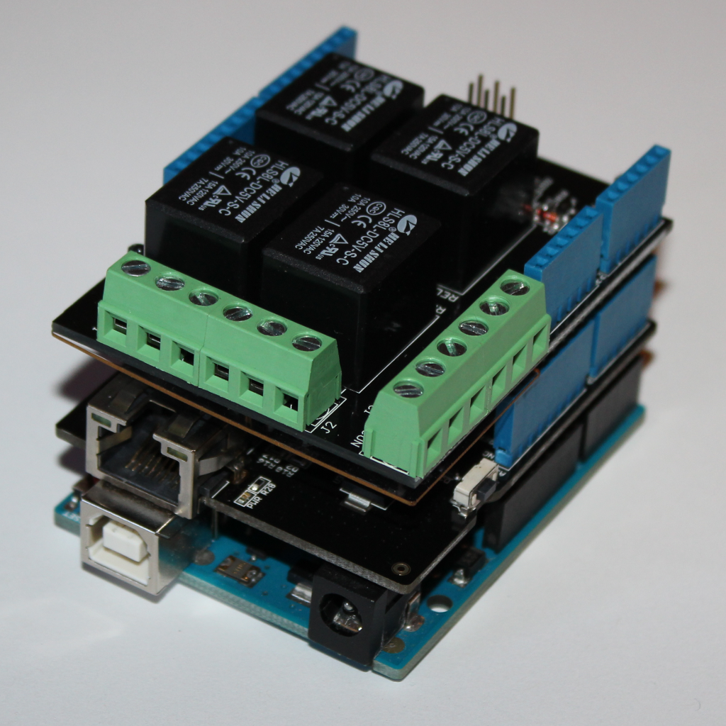
We had a few Halloween decorations with push button switches that we networked via an Arduino Uno. Three of the relays from the relay shield were used to activate a Grim Reaper and two sets of skulls. The push button from each decoration was cut and discarded. One of the wires coming from a decoration …
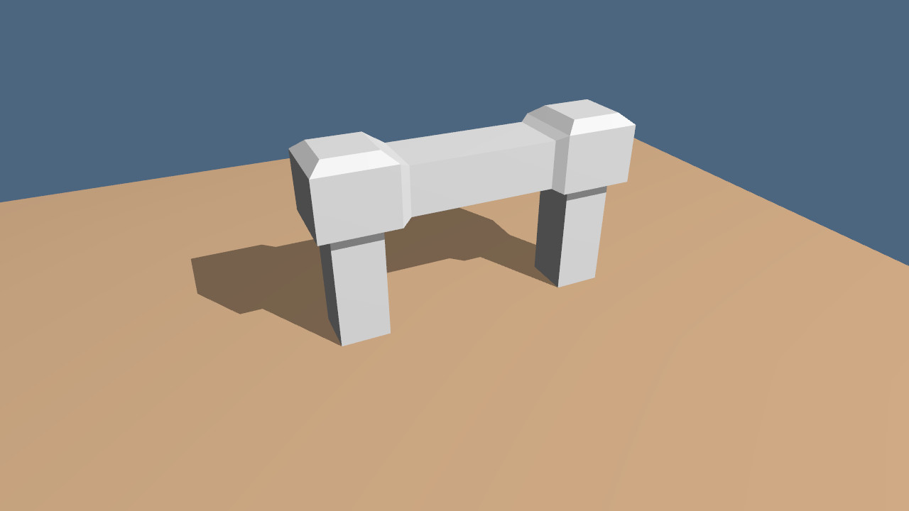
The purpose of this project was to provide a straightforward implementation of shadow volumes using the depth fail approach. The project is divided into the following sections: After loading an object, detect duplicate vertices. Build the object's edge list while identifying each face associated with an edge. Identify the profile edges from the perspective of …
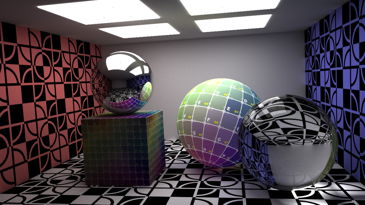
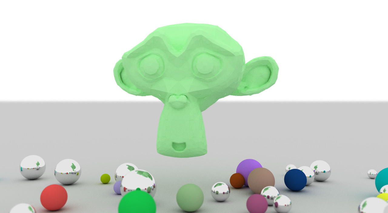
I had been planning to refine this project and offer a more detailed writeup on adding sphere and triangle texture mapping to the path tracer project, but for the time being I thought I would offer the code for download. Below are a couple of screen captures from the most recent version of the project. …
The equations for detecting features, tracking them between consecutive frames, and checking for consistency using an affine transformation will be derived below using the inverse compositional approach. We will begin by deriving the equations for tracking, because this will yield some insight into which features would be good to track. The source code for this …
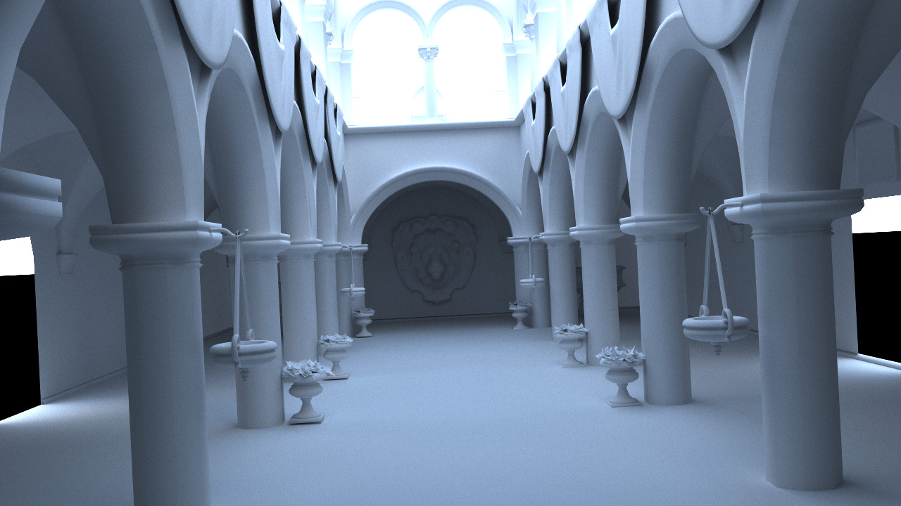
In this post we will employ the hyperplane separation theorem and the surface area heuristic for kd tree construction to improve the performance of our path tracer. Previous posts have relied simply on detecting intersections between an axis aligned bounding box and the minimum bounding box of a triangle primitive. By utilizing the hyperplane separation …
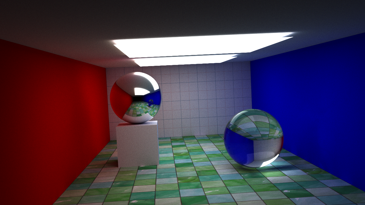
A few new features have been added to our path tracer. The depth of field extension has been reworked slightly using the thin lens equation allowing us to specify a focal length and aperture. Fresnel equations have been added to more accurately model the behavior of light at the interface between media of different refractive …
UPDATE: The post below was a purely naive attempt at implementing a rudimentary bounding volume hierarchy. A much more efficient implementation using a kd tree is available in this post. We will continue with the project we left off with in this post. We will attempt to add triangles to our list of primitives. Once …
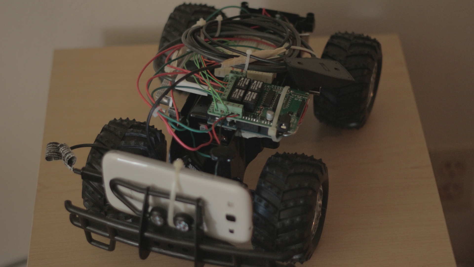
The purpose of this project was to create an internet-based rover using the combination of a cheap RC vehicle, an Arduino Uno with a Seeed Relay Shield, a Samsung Galaxy S3 in host mode, a workstation and PlayStation 3 controller. Our server software will run in the background on the S3 and visual feedback will …
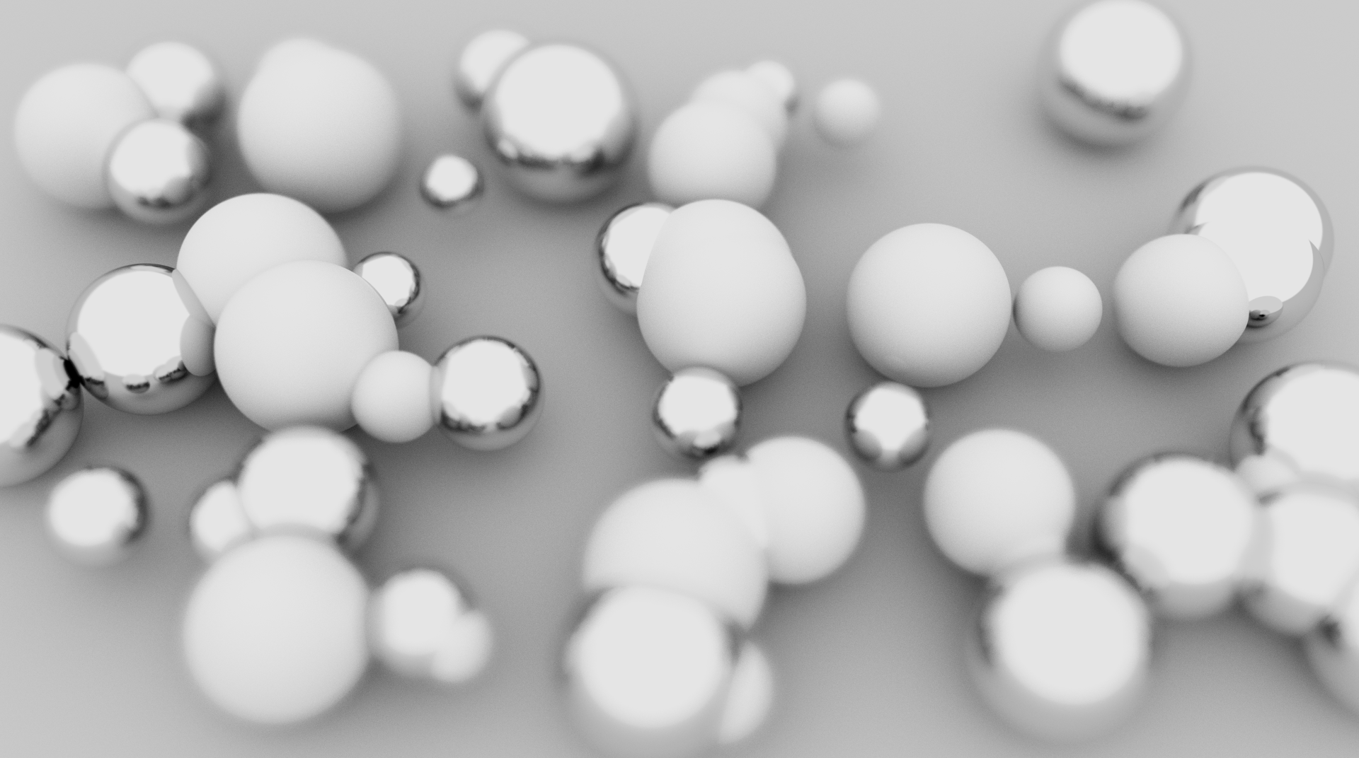
This is a small extension to the previous post. We will add a depth of field simulation to our path tracer project. I ran across this algorithm at this site. Below is a render of our path tracer with the depth of field extension. Essentially, we will define the distance to the focal plane and …

The path tracer we will create in this project will run on CUDA-enabled GPUs. You will need to install the CUDA Toolkit available from NVIDIA. The device code for this project uses classes and must be compiled with compute capability 2.0. If you are unsure what compute capability your card has, check out this list. …
The previous post was a discussion on employing Householder transformations to perform a QR decomposition. This post will be short. I've had this code lying around for a while now and thought I would make it available. The process of bidiagonalization using Householder transformations amounts to nothing more than alternating by left and right transformations. …
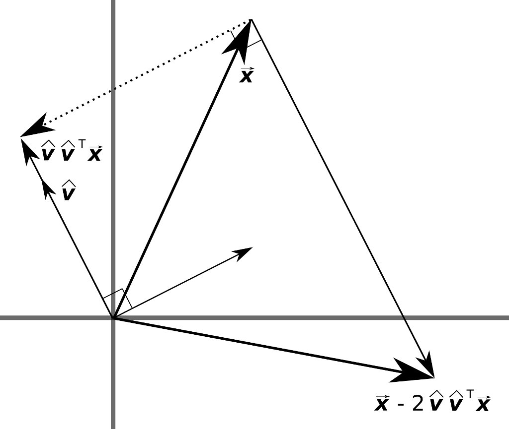
It's been a while since my last post. A project I have in the works requires some matrix decompositions, so I thought this would be a good opportunity to get a post out about QR decompositions using Householder transformations. For the moment we will focus on the field of real numbers, though we can extend …
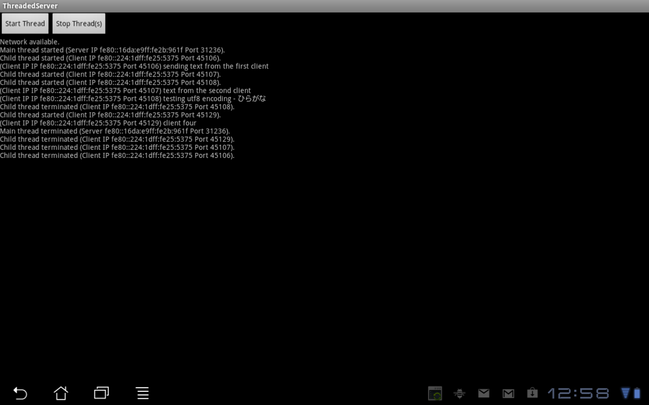
In this post we will create a basic concurrent server using threads in Java. The server will be implemented for the Android platform as part of a larger project to control a USB interface board remotely. Below are two screen captures. The first shows a state of the server after a few clients have connected …

In this post we will analyze the equations for the statistical wave model presented in Tessendorf's paper[1] on simulating ocean water. In the previous post we used the discrete Fourier transform to generate our wave height field. We will proceed with the analysis in order to implement our own fast Fourier transform. With this implementation …

In this post we will implement the statistical wave model from the equations in Tessendorf's paper[1] on simulating ocean water. We will implement this model using a discrete Fourier transform. In part two we will begin with the same equations but provide a deeper analysis in order to implement our own fast Fourier transform. Using …
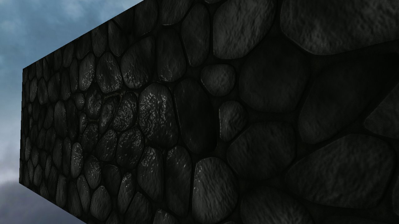
In the previous post we discussed lighting and environment mapping, and our evaluation of the lighting contribution was performed in view space. Here we will discuss lighting in tangent space and extend our lighting model to include a normal map. If we apply a texture to a surface, then for every point in the texture …

In this post we will expand on our skybox project by adding an object to our scene for which we will evaluate lighting contributions and environment mapping. We will first make a quick edit to our Wavefront OBJ loader to utilize OpenGL's Vertex Buffer Object. Once we can render an object we will create a …

I realized in my previous posts the use of OpenGL wasn't up to spec. This post will attempt to implement skybox functionality using the more recent specifications. We'll use GLSL to implement a couple simple shaders. We will create an OpenGL program object to which we will bind our vertex and fragment shaders. A Vertex …
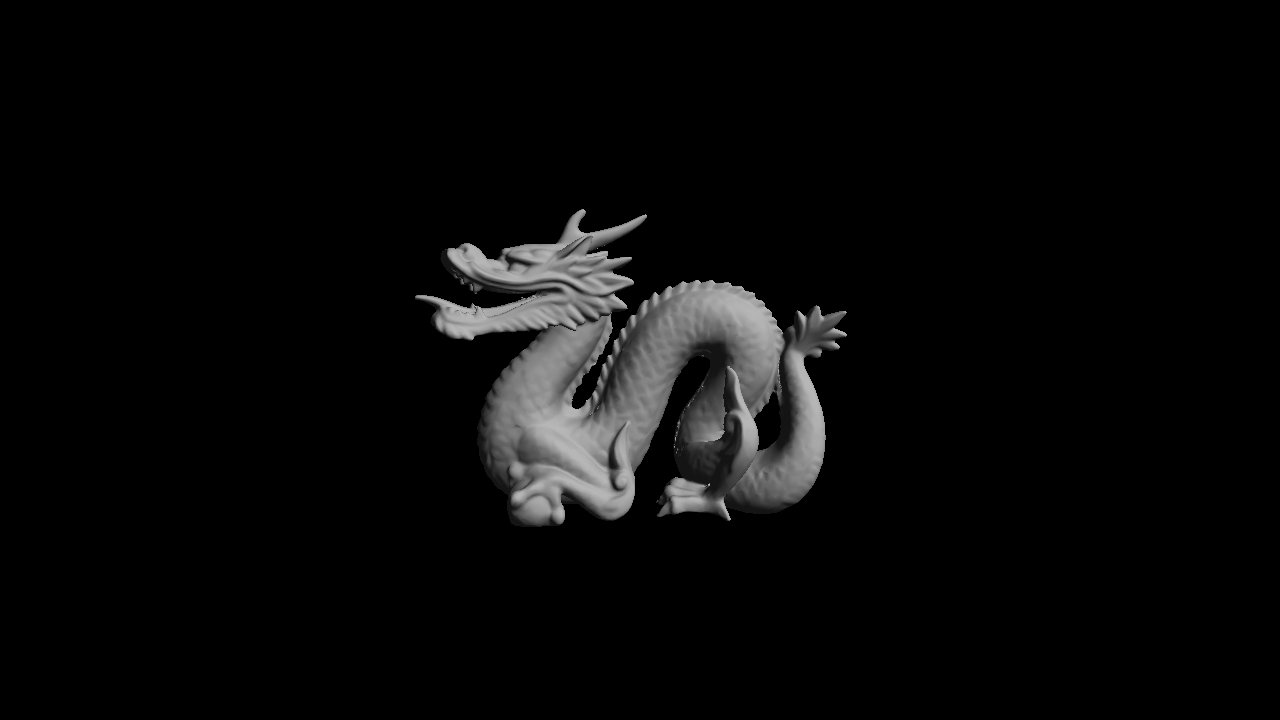
This post will examine the Wavefront OBJ file format and present a preliminary loader in C++. We will overlook the format's support for materials and focus purely on the geometry. Once our model has been loaded, an OpenGL Display List will be used to render the model. Below is a rendering of a dragon model …
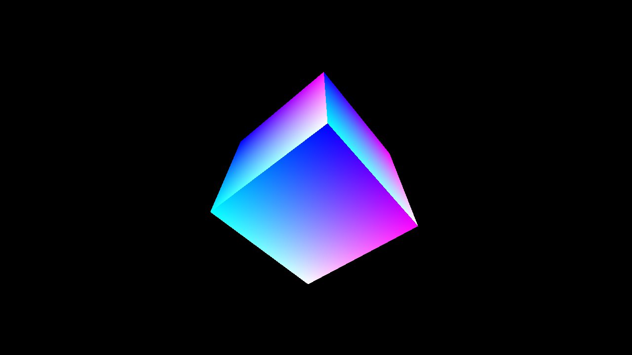
In this post we will construct a simple timer for evaluating the duration of a frame in addition to a keyboard handler. We will use these objects in conjunction to update our position relative to a cube. SDL and OpenGL will be used for rendering. Below is a frame captured from our application. We will …
In this post we will implement an object in C++ for accessing the state of an attached joystick. Below is a rendering using SDL and OpenGL of a joystick state. In "/usr/include/linux/joystick.h" we find the following event structure: Once we have opened a device node for reading we will populate this event structure with the …
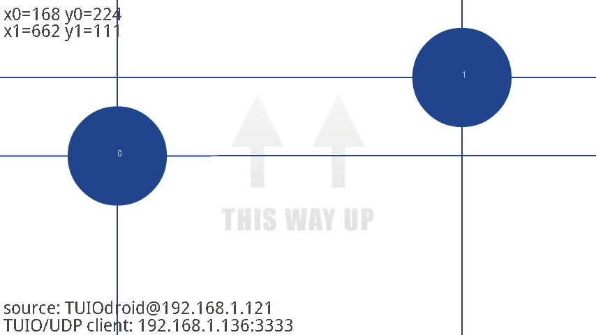
In this post we will begin to add TUIO (Tangible User Interface Object) support to our project by implementing a server module to parse OSC (Open Sound Control) packets for 2D cursor descriptions. This will allow us to import blob events from a client application. We will use the TUIOdroid application available for android devices …
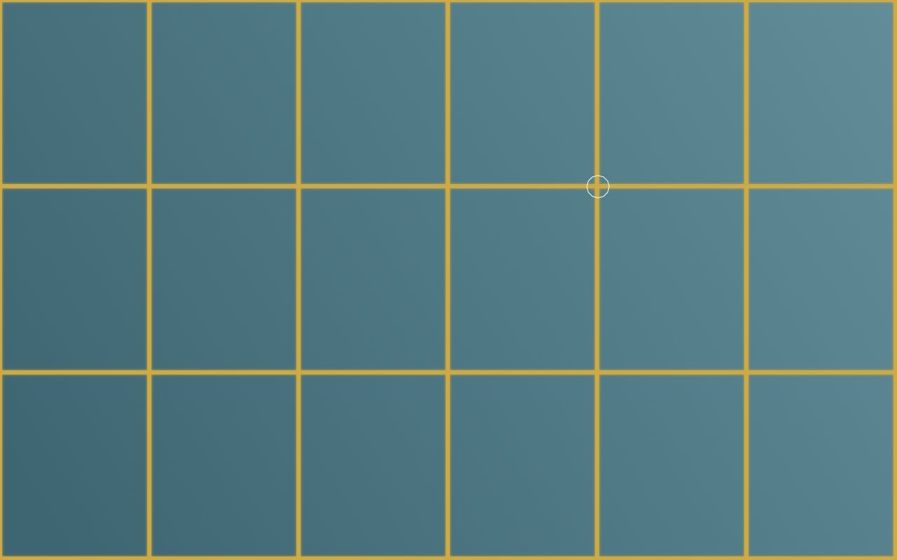
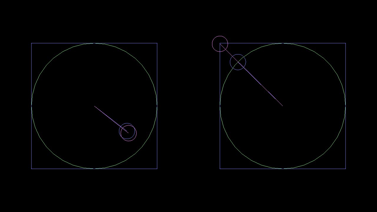
In this post we will touch upon the calibration component for multi-touch systems. By the end of this post we will implement a calibration widget that is integrated with our tracker modules, but before we do that we'll discuss the mathematics behind one method for mapping camera space to screen space. Below is a screen …

In the previous post we discussed the event queue and the abstract base class for the widgets. Now we will concentrate on creating some widgets that we can use by extending the base class, and we will look at setting up the queue, registering widgets, and calling the processEvents() method in our programs main loop. …
In my previous posts we've discussed blob extraction and tracking. Now we'll take it one step further and design an event system to handle those events and deliver them to registered widgets. In this post we will focus on the event system and the widget base class. In the next post we will extend the …
In the post before last we discussed using cvBlobsLib as a tool for blob extraction. We're going to revisit the extraction theme and look at a C++ implementation of the Connected Component Labeling method, but before we do that we're going to look at an implementation of the Disjoint Set data structure that will provide …
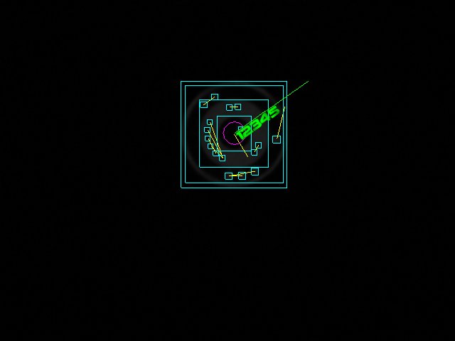
In my last post we discussed blob extraction and event tracking. We will continue with that project by adding support for two-dimensional fiducial tracking. We will attempt to implement the fiducial detection algorithm used on the Topolo Surface1. We will first describe the fiducials and how their properties are encoded in their structure, and we …
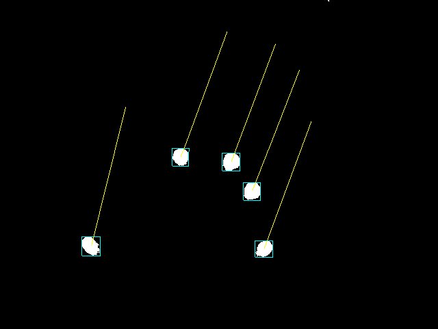
In my previous post we discussed using OpenCV to prepare images for blob detection. We will build upon that foundation by using cvBlobsLib to process our binary images for blobs. A C++ vector object will store our blobs, and the center points and axis-aligned bounding boxes will be computed for each element in this vector. …
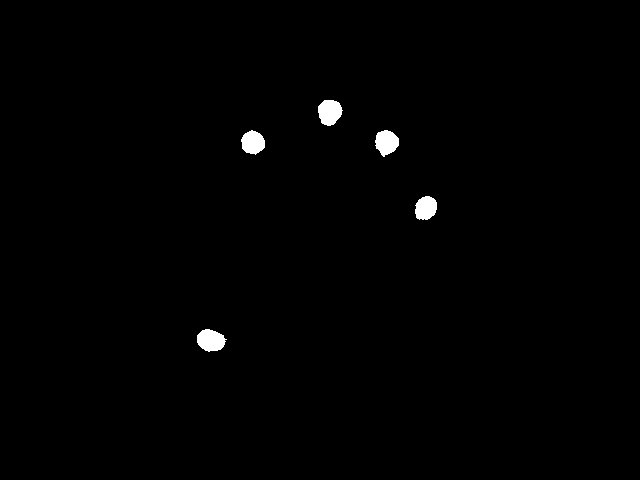
In this post I will discuss how you can capture and process images in preparation for blob detection. A future post will discuss the process of detecting and tracking blobs as well as fiducials, but here we are concerned with extracting clean binary images that will be passed to our detector module. We will use …